Segmentation of Stochastic Images using ... - Jacobs University

More documents

Recommendations

Info

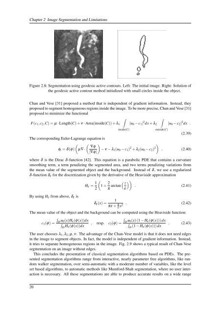
Chapter 2 Image Segmentation and Limitations Figure 2.8: Segmentation using geodesic active contours. Left: The initial image. Right: Solution of the geodesic active contour method initialized with small circles inside the object. Chan and Vese [31] proposed a method that is independent of gradient information. Instead, they proposed to segment homogeneous regions inside the image. To be more precise, Chan and Vese [31] proposed to minimize the functional ∫ ∫ F(c 1 ,c 2 ,C) = µ · Length(C) + ν · Area(inside(C)) + λ 1 |u 0 − c 1 | 2 dx + λ 2 |u 0 − c 2 | 2 dx . inside(C) The corresponding Euler-Lagrange equation is ( ( ) ) ∇φ φ t = δ(φ) µ∇ · − ν − λ 1 (u 0 − c 1 ) 2 + λ 2 (u 0 − c 2 ) 2 |∇φ| outside(C) (2.39) , (2.40) where δ is the Dirac δ-function [42]. This equation is a parabolic PDE that contains a curvature smoothing term, a term penalizing the segmented area, and two terms penalizing variations from the mean value of the segmented object and the background. Instead of δ, we use a regularized δ-function δ ε for the discretization given by the derivative of the Heaviside approximation H ε = 1 ( 1 + 2 ( z ) ) 2 π arctan . (2.41) ε By using H ε from above, δ ε is 1 δ ε (x) = πε + π . (2.42) ε x2 The mean value of the object and the background can be computed using the Heaviside function: ∫ D c 1 (φ) = u ∫ 0(x)H ε (φ(x))dx ∫ D D H , resp. c 2 (φ) = u 0(x)(1 − H ε (φ(x)))dx ∫ ε(φ(x))dx D (1 − H . (2.43) ε(φ(x)))dx The user chooses λ 1 ,λ 2 , µ,ν. The advantage of the Chan-Vese model is that it does not need edges in the image to segment objects. In fact, the model is independent of gradient information. Instead, it tries to separate homogeneous regions in the image. Fig. 2.9 shows a typical result of Chan-Vese segmentation on an image without edges. This concludes the presentation of classical segmentation algorithms based on PDEs. The presented segmentation algorithms range from interactive, nearly parameter free algorithms, like random walker segmentation, over semi-automatic with a moderate number of variables, like the level set based algorithms, to automatic methods like Mumford-Shah segmentation, where no user interaction is necessary. All these segmentations are able to produce accurate results on a wide range 20
2.5 Why is Classical Image Processing not Enough? Figure 2.9: Segmentation of an object without sharp edges using the Chan-Vese approach. In red, we show the steady-state solution of the Chan-Vese segmentation method initialized with a small circle inside the object. of images and from the perspective of segmentation of single images, there is no need for new concepts. Nevertheless, the approaches presented in this chapter have drawbacks regarding robustness with respect to noise, reproducibility, and error propagation. The next section investigates this. 2.5 Why is Classical Image Processing not Enough? In the last sections, we introduced five segmentation methods and showed that all these segmentation methods perform well on some selected medical images. Besides the segmentation of single images, a segmentation method has to fulfill other features not presented so far: • It is unclear how robust the methods are with respect to image noise. • The robustness of the methods for parameter changes and different initializations is unclear. • Propagating error information through these algorithms is hard, i.e. if information about measurement errors at the image acquisition is available, it is impossible to propagate this information through the segmentation to get segmentation results containing the error information. We organized this section as follows: First, we give an introduction to image noise, show how the image noise influences the image quality for different acquisition modalities and how image noise is modeled mathematically. Then, we investigate the noise robustness of the presented segmentation methods, and finally, we discuss error propagation in classical image segmentation methods. 2.5.1 Image Noise Image noise is a serious problem when dealing with medical images and images from digital cameras. Different noise sources degrade the images. A principal problem of image acquisition devices is the noise due to the random arrival of the photons. Light or X-ray emission is a stochastic process [44]. In addition, the instrumentation noise due to thermal effects in the acquisition device degrades the image quality. Further sources of image noise are the quantization noise due to the conversion from analog to digital signals and the compression process for the images, if any. Physical effects influencing the path of the photons, like blurring, diffraction, and scattering, cause image noise, too. 21
Page 1: Segmentation of Stochastic Images u
Page 5: Abstract The task of segmentation,
Page 8 and 9: 7.5 Segmentation of Stochastic Imag
Page 11 and 12: Chapter 1 Introduction The developm
Page 13 and 14: Figure 1.3: This thesis combines fi
Page 15: the presentation of the stochastic
Page 18 and 19: Chapter 2 Image Segmentation and Li
Page 36 and 37: Chapter 3 SPDEs and Polynomial Chao
Page 48 and 49: Chapter 4 Discretization of SPDEs F
Page 50 and 51: Chapter 4 Discretization of SPDEs 4
Page 52 and 53: Chapter 4 Discretization of SPDEs a
Page 58 and 59: Chapter 5 Stochastic Images
Page 60 and 61: Chapter 5 Stochastic Images Figure
Page 62 and 63: Chapter 5 Stochastic Images like qu
Page 64 and 65: Chapter 5 Stochastic Images Figure
Page 67 and 68: Chapter 6 Segmentation of Stochasti
Page 69 and 70: 6.1 Random Walker Segmentation on S
Page 77 and 78: 6.2 Ambrosio-Tortorelli Segmentatio
Page 79 and 80: 6.2 Ambrosio-Tortorelli Segmentatio
Page 81 and 82:
6.2 Ambrosio-Tortorelli Segmentatio
Page 83 and 84:
Page 85 and 86:
Page 87:
Page 90 and 91:
Chapter 7 Stochastic Level Sets whe
Page 92 and 93:
Chapter 7 Stochastic Level Sets Fig
Page 94 and 95:
Chapter 7 Stochastic Level Sets and
Page 96 and 97:
Chapter 7 Stochastic Level Sets rar
Page 98 and 99:
Page 100 and 101:
Chapter 7 Stochastic Level Sets MC
Page 102 and 103:
Page 104 and 105:
Page 106 and 107:
Chapter 7 Stochastic Level Sets act
Page 108 and 109:
Chapter 8 Segmentation of Classical
Page 110 and 111:
Page 112 and 113:
Page 114 and 115:
Page 116 and 117:
Page 118 and 119:
Chapter 9 Summary, Discussion, and
Page 121 and 122:
List of Figures 1.1 Left: CT image
Page 123 and 124:
List of Figures 6.2 Mean and varian
Page 125:
List of Figures 7.12 Mean (left) of
Page 129 and 130:
Appendix A Publications Written Dur
Page 131 and 132:
Bibliography [14] L. Ambrosio and M
Page 133 and 134:
Bibliography [46] B. Echebarria, R.
Page 135 and 136:
Bibliography [81] B. N. Khoromskij
Page 137 and 138:
Bibliography [113] A. Nouy. A gener
Page 139:
Bibliography [147] J. Tryoen, O. Le
show all

Segmentation of Stochastic Images using ... - Jacobs University

You also want an ePaper? Increase the reach of your titles

Delete template?

Save as template?