Segmentation of Stochastic Images using ... - Jacobs University

More documents

Recommendations

Info

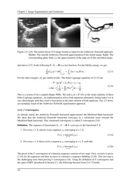
Chapter 2 Image Segmentation and Limitations Figure 2.5: Left: The initial (noisy) US image treated as input for the Ambrosio-Tortorelli approach. Middle: The smooth Ambrosio-Tortorelli approximation of the initial image. Right: The corresponding phase field, i.e. the approximation of the edge set of the smoothed image. derivatives [17]. In the following θ : D → IR is a test function. For the fidelity energy, we get: d dε E ∫ f id[u + εθ] ∣ = 2(u + u 0 )θ dx . (2.17) ε=0 For the other energies, we get similar results. The Euler-Lagrange equations of (2.15) are D −∇ · (µ(φ 2 + k ε )∇u ) + u = u 0 ( 1 −ε∆φ + 4ε + µ ) 2ν |∇u|2 φ = 1 4ε . (2.18) This is a system of two coupled elliptic PDEs. We seek u,φ ∈ H 1 (D) as the weak solutions of these Euler-Lagrange equations. An implementation solves both equations alternately, letting either u or φ vary alternatingly until they reach a fixed point as the joint solution of both equations. Fig. 2.5 shows an exemplary result of the Ambrosio-Tortorelli segmentation approach. 2.3.2 Γ-Convergence As already stated, the Ambrosio-Tortorelli functional approximates the Mumford-Shah functional. We show that the Ambrosio-Tortorelli functional converges in a variational sense towards the Mumford-Shah functional. This variational convergence is called Γ-convergence [14]: Definition The sequence of functionals F n : X → IR Γ-converges to the functional F if 1. For every x ∈ X and for every sequence x n converging to x ∈ X, F(x) ≤ liminf n→∞ F n(x n ) . (2.19) 2. For every x ∈ X there exists a sequence x n converging to x ∈ X such that F(x) ≥ limsupF n (x n ) . (2.20) n→∞ The proof of the Γ-convergence of a function sequence consists of two steps: First, we have to prove (2.19) for all sequences and then we have to construct a sequence fulfilling (2.20). This last step is the challenging task when proving Γ-convergence [14]. Using the definition of Γ-convergence and the space GSBV introduced in Section 2.1, the following theorem from [14, 17] holds. 14
2.3 Mumford-Shah and Ambrosio-Tortorelli Segmentation Theorem 2.1. Define Ẽ AT : L 1 (D) × L 1 (D) → IR + by { EAT (u,φ) if (u,φ) ∈ H Ẽ AT (u,φ) := 1 (D) × H 1 (D),0 ≤ φ ≤ 1 +∞ otherwise (2.21) and G : L 1 (D) × L 1 (D) → IR + by { EMS (u) if u ∈ GSBV(D) and φ = 1 almost everywhere G(u,φ) = +∞ otherwise. (2.22) If k ε = o(ε), then Ẽ AT Γ-converges to G(u,φ) for ε → 0. The convergence of the Ambrosio-Tortorelli energy towards the Mumford-Shah energy enables us to use the coupled pair of PDEs obtained as Euler-Lagrange equations of the Ambrosio-Tortorelli energy and to solve this with very small ε. The result is a phase field that is close to the characteristic function of the edge set of the Mumford-Shah functional. 2.3.3 Edge Continuity and Edge Consistency The classical Mumford-Shah model and the Ambrosio-Tortorelli approximation lack a step linking edges. This step is necessary to enforce the detection of closed contours in the images. Otherwise, the appearance of partially detected, breaking up contours is possible, see Fig. 2.5. For example, Erdem et al. [49] introduced such a step for the Ambrosio-Tortorelli model. The idea is to use a modified diffusion coefficient in the image equation. This modified coefficient does not depend on the phase field exclusively, but contains information about the continuity and directional consistency of the detected edges. To be more precise, Erdem et al. [49] proposed to use the equation −∇ · (µ((cφ) 2 + k ε )∇u ) + u = u 0 , (2.23) instead of the first equation of (2.18). The additional factor c is the product of the two factors from the directional consistency c dc and the edge continuity c h , i.e. c = c dc · c h . (2.24) If c < 1, the diffusivity decreases, allowing to form new edges in the image, whereas c > 1 leads to an increased diffusivity, allowing to smooth away unwanted edges. Directional Consistency The directional consistency tries to judge the quality of the detected edges based on information from surrounding pixels. The idea is that an edge is reliable if the gradients of the image for pixels in directions perpendicular to the edge are in parallel. For inaccurately detected edges, e.g. due to noise, these gradients are typically not aligned. To do so, Erdem et al. [49] introduced (c dc ) i = ζ dc i + 1 − ζ i dc (2.25) φ i for all pixels i ∈ I , where ζi dc measures the alignment of the gradients. This factor increases the diffusion, if the image gradients around the detected edge are not aligned. As the feedback measure for the alignment of the gradients they proposed to use ( ( )) 1 ζi dc = exp ε dc |η s | ∑ ∇v j∈η s i · ∇v j − 1 , (2.26) 15
Page 1: Segmentation of Stochastic Images u
Page 5: Abstract The task of segmentation,
Page 8 and 9: 7.5 Segmentation of Stochastic Imag
Page 11 and 12: Chapter 1 Introduction The developm
Page 13 and 14: Figure 1.3: This thesis combines fi
Page 15: the presentation of the stochastic
Page 18 and 19: Chapter 2 Image Segmentation and Li
Page 36 and 37: Chapter 3 SPDEs and Polynomial Chao
Page 48 and 49: Chapter 4 Discretization of SPDEs F
Page 50 and 51: Chapter 4 Discretization of SPDEs 4
Page 52 and 53: Chapter 4 Discretization of SPDEs a
Page 58 and 59: Chapter 5 Stochastic Images
Page 60 and 61: Chapter 5 Stochastic Images Figure
Page 62 and 63: Chapter 5 Stochastic Images like qu
Page 64 and 65: Chapter 5 Stochastic Images Figure
Page 67 and 68: Chapter 6 Segmentation of Stochasti
Page 69 and 70: 6.1 Random Walker Segmentation on S
Page 75 and 76:
6.1 Random Walker Segmentation on S
Page 77 and 78:
6.2 Ambrosio-Tortorelli Segmentatio
Page 79 and 80:
Page 81 and 82:
Page 83 and 84:
Page 85 and 86:
Page 87:
Page 90 and 91:
Chapter 7 Stochastic Level Sets whe
Page 92 and 93:
Chapter 7 Stochastic Level Sets Fig
Page 94 and 95:
Chapter 7 Stochastic Level Sets and
Page 96 and 97:
Chapter 7 Stochastic Level Sets rar
Page 98 and 99:
Page 100 and 101:
Chapter 7 Stochastic Level Sets MC
Page 102 and 103:
Page 104 and 105:
Page 106 and 107:
Chapter 7 Stochastic Level Sets act
Page 108 and 109:
Chapter 8 Segmentation of Classical
Page 110 and 111:
Page 112 and 113:
Page 114 and 115:
Page 116 and 117:
Page 118 and 119:
Chapter 9 Summary, Discussion, and
Page 121 and 122:
List of Figures 1.1 Left: CT image
Page 123 and 124:
List of Figures 6.2 Mean and varian
Page 125:
List of Figures 7.12 Mean (left) of
Page 129 and 130:
Appendix A Publications Written Dur
Page 131 and 132:
Bibliography [14] L. Ambrosio and M
Page 133 and 134:
Bibliography [46] B. Echebarria, R.
Page 135 and 136:
Bibliography [81] B. N. Khoromskij
Page 137 and 138:
Bibliography [113] A. Nouy. A gener
Page 139:
Bibliography [147] J. Tryoen, O. Le
show all

Segmentation of Stochastic Images using ... - Jacobs University

You also want an ePaper? Increase the reach of your titles

Delete template?

Save as template?