Segmentation of Stochastic Images using ... - Jacobs University

3.4 Relation to Interval Arithmetic
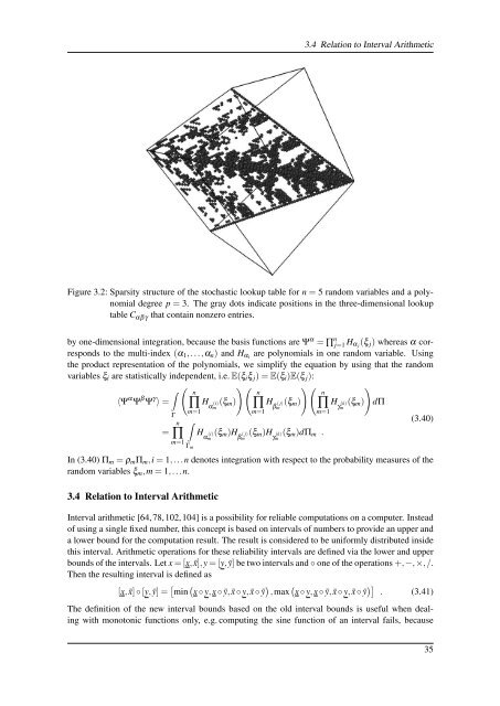
Figure 3.2: Sparsity structure of the stochastic lookup table for n = 5 random variables and a polynomial
degree p = 3. The gray dots indicate positions in the three-dimensional lookup
table C αβγ that contain nonzero entries.
by one-dimensional integration, because the basis functions are Ψ α = ∏ n j=1 H α j
(ξ j ) whereas α corresponds
to the multi-index (α 1 ,...,α n ) and H αi are polynomials in one random variable. Using
the product representation of the polynomials, we simplify the equation by using that the random
variables ξ i are statistically independent, i.e. E(ξ i ξ j ) = E(ξ i )E(ξ j ):
)
∫
〈Ψ α Ψ β Ψ γ 〉 =
dΠ
=
Γ
n
∏
m=1
(
n
∏
m=1
∫
H (i) α m
Γ m
n
H (i) α
(ξ m ))(
∏
m
m=1
(ξ m )H β
( j)
m
n
H ( j) β
(ξ m ))(
∏
m
m=1
(ξ m )H (k) γ
(ξ m )dΠ m .
m
H (k) γ
(ξ m )
m
(3.40)
In (3.40) Π m = ρ m Π m ,i = 1,...n denotes integration with respect to the probability measures of the
random variables ξ m ,m = 1,...n.
3.4 Relation to Interval Arithmetic
Interval arithmetic [64,78,102,104] is a possibility for reliable computations on a computer. Instead
of using a single fixed number, this concept is based on intervals of numbers to provide an upper and
a lower bound for the computation result. The result is considered to be uniformly distributed inside
this interval. Arithmetic operations for these reliability intervals are defined via the lower and upper
bounds of the intervals. Let x = [x, ¯x],y = [y,ȳ] be two intervals and ◦ one of the operations +,−,×,/.
Then the resulting interval is defined as
[x, ¯x] ◦ [y,ȳ] = [ min ( x ◦ y,x ◦ ȳ, ¯x ◦ y, ¯x ◦ ȳ ) ,max ( x ◦ y,x ◦ ȳ, ¯x ◦ y, ¯x ◦ ȳ )] . (3.41)
The definition of the new interval bounds based on the old interval bounds is useful when dealing
with monotonic functions only, e.g. computing the sine function of an interval fails, because
35