- Page 1 and 2:
c,q /kao, PROPERTY OF THF H S. GOVE
- Page 3 and 4:
INSTITUTE FOR WATER RESOURCES In 19
- Page 5 and 6:
NORTHWESTERN UNIVERSITY AN ECONOMET
- Page 7 and 8:
ACKNOWLEDGMENTS LIST OF FIGURES •
- Page 9 and 10:
Figure FIGURES Page 3.1 Two-Market
- Page 11 and 12:
Table Page 4.12 Rail Rate Regressio
- Page 13 and 14:
Table 4.A.5 Rate Regression Rail Qu
- Page 15 and 16:
This paper presents an economic mod
- Page 17 and 18:
All transport modes are designed to
- Page 19 and 20:
CHAPTER II REVIEW OF THE LITERATURE
- Page 21 and 22:
The first significant generalizatio
- Page 23 and 24:
artificially contrived solution met
- Page 25 and 26:
trannportnLion, thin neglect ham cP
- Page 27 and 28:
to the mode under consideration, cr
- Page 29 and 30:
that even if the reasoning is 'corr
- Page 31 and 32:
competition, that is where the qual
- Page 33 and 34:
His estimating process is divided i
- Page 35 and 36:
Table 2.1 COMMODITIES CARRIED ON TH
- Page 37 and 38:
- 15 In a recent volume on the de=a
- Page 39 and 40:
aggregation over regions for each c
- Page 41 and 42:
for each of the modes under the ass
- Page 43 and 44:
ail rates, and here he encountered
- Page 45 and 46:
had statistical significance; howev
- Page 47 and 48:
flows with actual shipments. 21 The
- Page 49 and 50:
CHAPTER III THE TWO-MARKET MULTI-MO
- Page 51 and 52:
the market price in A it is obvious
- Page 53 and 54:
P b P o P a T r 0 Fig. 3.4 -- Equil
- Page 55 and 56:
for all quantities, we conceive of
- Page 57 and 58:
0 (3.6.A) (3.6.B) Q 2 Fig. 3.6 -- T
- Page 59 and 60:
• Q2 Qi Q0 Fig. 3.7 -- Two-Mode M
- Page 61 and 62:
preference. He pays money today for
- Page 63 and 64:
Situation II: Producer Ownership. T
- Page 65 and 66:
little consideration will reveal th
- Page 67 and 68:
considered these costs in several f
- Page 69 and 70:
Then, to calculate the rate of chan
- Page 71 and 72:
(T1) (T2) The effect upon Q of an i
- Page 73 and 74:
(3.A.7) (3.A.8) APPENDIX A TO CHAPT
- Page 75 and 76:
(3.A.17) (3.A.18) ■FQ 5-(43-- -7,
- Page 77 and 78:
term more negative and, since it is
- Page 79 and 80:
and its inverse (3.B.8) T c • C(Q
- Page 81 and 82:
Now, going back to equation (3.3.7)
- Page 83 and 84:
APPENDIX C TO CHAPTER THREE The Two
- Page 85 and 86:
product to be transported, Q1 units
- Page 87 and 88:
(3.C. 3) ,(3.C.6) The monopolist's
- Page 89 and 90:
To obtain the greatest profits, the
- Page 91 and 92:
.1., OA The sign of — is only sli
- Page 93 and 94:
(4.11) (4.12) (4.13) (4.14) 111 Tc
- Page 95 and 96:
(4.26) (4.27) (4.28) (4.29) (4.30)
- Page 97 and 98:
The tons figure is the total tonnag
- Page 99 and 100:
Since the aim of this study is to e
- Page 101 and 102:
Distance ' Quantity Rate Eq. (4.33)
- Page 103 and 104:
Distance Quantity Rate Eq. (4.33) (
- Page 105 and 106:
Distance Quantity Rate Eq. , Source
- Page 107 and 108:
Distance Quantity Rate . Eq. Distan
- Page 109 and 110:
where R E average, revenue received
- Page 111 and 112:
• Table 4.8 332.42 808.54 478.58
- Page 113 and 114:
269.02 931.44 900.75 0.98 0.98 0.97
- Page 115 and 116:
Table 4.12 RAIL RATE REGRESSIONS FI
- Page 117 and 118:
1. date of the freight bill. 2. ori
- Page 119 and 120:
(4.41) Rik ■ 0 30 + 0 31 Mik + 0
- Page 121 and 122:
making is usually taken to refer to
- Page 123 and 124:
Total 728 79,603 Reduction due to m
- Page 125 and 126:
Source of Variance Total Reduction
- Page 127 and 128:
there is a wide difference between
- Page 129 and 130:
All Commodity Classes. Table 4.20 c
- Page 131 and 132:
Source of Variance Total 100 599,25
- Page 133 and 134:
Intercept Distance Quantity Density
- Page 135 and 136:
Intercept Distance Quantity Density
- Page 137 and 138:
stability and density showed very l
- Page 139 and 140:
groups into STCC commodity groups,
- Page 141 and 142:
The reduced form of this system is
- Page 143 and 144:
Exogenous , Changes(X) Transport de
- Page 145 and 146:
the quantity of commodity k transpo
- Page 147 and 148:
Regression Distance < 200 mi. Rail
- Page 149 and 150:
Regression Distance Rail Motor Dist
- Page 151 and 152:
increase with distances. This is ra
- Page 153 and 154:
Table 4.33 contains the derived rat
- Page 155 and 156:
Sample Regression Size Intercept M2
- Page 157 and 158:
Mode Int. Mode Sample Size Rate Tab
- Page 159 and 160:
Mode Sample Size Table 4.38 STCC 32
- Page 161 and 162:
Sample Regression Size Intercept Di
- Page 163 and 164:
Table 4.42 STCC 37 - TRANSPORTATION
- Page 165 and 166:
the three-mode model. Table 4.43 di
- Page 167 and 168:
Summary of the Empirical Results In
- Page 169 and 170:
Table 4.45 FREIGHT RATE DATA ANALYS
- Page 171 and 172:
Commodity Group II III IV V Total C
- Page 173 and 174:
Group Mode . I Truck Rail Water /I
- Page 175 and 176:
shipments. After a lengthy analysis
- Page 177 and 178:
for Group III is positive, large an
- Page 179 and 180:
of the underlying structural parame
- Page 181 and 182:
Table 4.49 DEMAND REGRESSIONS FINAL
- Page 183 and 184:
• supply The model assumes that t
- Page 185 and 186:
Commodity Group Table 4.50 DEMAND A
- Page 187 and 188:
APPENDIX A TO CHAPTER FOUR The Effe
- Page 189 and 190:
Table 4.A.2 RATE REGRESSION RAIL QU
- Page 191 and 192:
Table 4.A.4 RATE REGRESSION RAIL QU
- Page 193 and 194:
The overall tendency appears to be
- Page 195 and 196:
CHAPTER V SUMMARY AND CONCLUSIONS R
- Page 197 and 198:
theoretical basis for their empiric
- Page 199 and 200:
competitive industries. Applying th
- Page 201 and 202:
in the appendix to that chapter. Th
- Page 203 and 204:
BIBLIOGRAPHY Baumol, W. J., "Calcul
- Page 205 and 206:
United States Department of Commerc
- Page 207 and 208:
NORTHWESTERN UNIVERSITY A MODEL OF
- Page 209 and 210:
CHAPTER IV EMPIRICAL RESULTS . Page
- Page 211 and 212:
. INTRODUCTION Our goal is to study
- Page 213 and 214:
Other studies have been done by the
- Page 215 and 216:
. Recently air freight has grown aw
- Page 217 and 218:
• For instance, suppose a firm ha
- Page 219 and 220:
eceive the same criticisms as above
- Page 221 and 222:
Per Cent WA Decrease From Current L
- Page 223 and 224:
• Cargo . Brewer's analysis depen
- Page 225 and 226:
A different type of approach, is ta
- Page 227 and 228:
These substantial estimates of elas
- Page 229 and 230:
and the consumption points. These a
- Page 231 and 232:
Initially, the determinants of a fi
- Page 233 and 234:
axis. Q is the quantity the firm wo
- Page 235 and 236:
Arc elasticity of the associated tr
- Page 237 and 238:
• same A*es (-p)/-11 Skto 4441.
- Page 239 and 240:
Suppose that the range of one choic
- Page 241 and 242:
is better than getting P 2 tomorrow
- Page 243 and 244:
A, At the kink P . Any_further rais
- Page 245 and 246:
market price; or inventory costs ma
- Page 247 and 248:
The shipper must pay a transport bi
- Page 249 and 250:
quantity transported of Z decreases
- Page 251 and 252:
The analysis yields a downward slop
- Page 253 and 254:
of each market and calculates each
- Page 255 and 256:
If more consumption points ,are add
- Page 257 and 258:
or ( 5 1) . 1. Q-14.)4 `("P)EXarg (
- Page 259 and 260:
4. 0 -A? 040- Net MR 1 0 so. Ira."
- Page 261 and 262:
To determine the demand curve for t
- Page 263 and 264:
I • The above equations (1-4) wer
- Page 265 and 266:
(I). 1■1 (7). Id. (8). •a 0.0.1
- Page 267 and 268:
• goods arrive (so that Q A+Q S g
- Page 269 and 270:
k The optimal amounts of QA and Q s
- Page 271 and 272:
it has been used in economics. Basi
- Page 273 and 274:
An analogous relationship exists fo
- Page 275 and 276:
• • (11). Now a probability dis
- Page 277 and 278:
--_.—..---...........AawmarA D SA
- Page 279 and 280:
, (1). APPENDIX TO CHAPTER III SENS
- Page 281 and 282:
decreases. Proper choice of P rA (X
- Page 283 and 284:
products, have different cost funct
- Page 285 and 286:
The above data falls short of the q
- Page 287 and 288:
lower than air rates. It rises more
- Page 289 and 290:
One of the objectives of the study
- Page 291 and 292:
a. Regression equation TABLE IV-1 r
- Page 293 and 294:
significant. 8 It was, therefore, d
- Page 295 and 296:
in large tonnages tend to have a lo
- Page 297 and 298:
T .A T ° S Highest value per pound
- Page 299 and 300:
. In addition, only the smallest qu
- Page 301 and 302:
Here the deviations are zero. The r
- Page 303 and 304:
certain range, the demand estimates
- Page 305 and 306:
expected as goods in the discrimina
- Page 307 and 308:
• BIBLIOGRAPHY [1] Air Cargo Maga
- Page 309 and 310:
[24] 2 Study of the Possibilities f
- Page 311 and 312:
[42] Dawson, Michael, "A Technique
- Page 313 and 314:
[62] Gorham, G., Sealy, K.R. 1 and
- Page 315 and 316:
■•■•■■•••••
- Page 317 and 318:
[100] Richards, Anthony, The Role o
- Page 319 and 320:
[120] Traffic World Marketing Study
- Page 321 and 322:
! i \ NORTHWESTERN UNIVERSITY FREIG
- Page 323 and 324:
While working on this dissertation
- Page 325 and 326:
BIBLIOGRAPHY Anderson, T.W. "An Int
- Page 327 and 328:
VITA MICHEL VINCENT BEUTHE Born in
- Page 329 and 330:
of cost iv iazroduced at once along
- Page 331 and 332:
In the present theoretical formulat
- Page 333 and 334:
It is possible to generalize this m
- Page 335 and 336:
however, because of their nature, t
- Page 337 and 338:
ij xo ij ,Diagram 3, . 0 X ij of th
- Page 339 and 340:
equal to+ where E is the median of
- Page 341 and 342:
CHAPTER II Discrimination With One
- Page 343 and 344:
which is,.in this case, the only q
- Page 345 and 346:
Notc that the first subscript of a.
- Page 347 and 348:
I .' 1) (22) P 1 (X) = (25) Therefo
- Page 349 and 350:
(34) P 2 (X) (36) 1 = 1 a b c ' and
- Page 351 and 352:
CHAPTER III An Application - Corn T
- Page 353 and 354:
time the draft is honored by the co
- Page 355 and 356:
2. Critique of the Data. We must no
- Page 357 and 358:
made through questionnaires to coun
- Page 359 and 360:
we can still hope to obtain satisfa
- Page 361 and 362:
common and contract carriers are co
- Page 363 and 364:
Table II. Rail Time Regressions: Ti
- Page 365 and 366:
3. The Statistical Results. After t
- Page 367 and 368:
Table IV gives the discriminant fun
- Page 369 and 370: February non-weighed July weighed T
- Page 371 and 372: the binary problems, when the choic
- Page 373 and 374: Table VII Probabilities that an obs
- Page 375 and 376: Table VIII, Probability of Correct
- Page 377 and 378: significantly different from the 'n
- Page 379 and 380: -X _21 5.15 L4.45 TRUCK RAIL lalm
- Page 381 and 382: CHAPTER IV. A Predictive Model of R
- Page 383 and 384: C ab /C a is smaller than one, the
- Page 385 and 386: II. Rail-Water Competition: One Por
- Page 387 and 388: Until now, no attention has been pa
- Page 389 and 390: 9 ) (Z a - kZ b ) = C w /C r Zab +
- Page 391 and 392: shipper. In the reality of competit
- Page 393 and 394: DIAGRAM 5 For the most interesting
- Page 395 and 396: DIAGRAM 7 waterway may be numerous.
- Page 397 and 398: Note the restriction of Y to its ab
- Page 399 and 400: the road-water route. In (24) C t (
- Page 401 and 402: Squaring both sides, one obtains an
- Page 403 and 404: interesting expressions. However, t
- Page 405 and 406: CHAPTER V. This chapter attempts to
- Page 407 and 408: TOTAL . COST D = -(L r - L t ) 2 Th
- Page 409 and 410: 2. Two Markets Model. subject --co
- Page 411 and 412: X 0, X 2 - 0. It can readily be see
- Page 413 and 414: the river does not have any --, but
- Page 415 and 416: :sLY: x rail 0 truck 0 rail and tru
- Page 417 and 418: 'NLY: K rail 0 truck 0 rail and tru
- Page 419: Table XI. Rail Rates Regressions: C
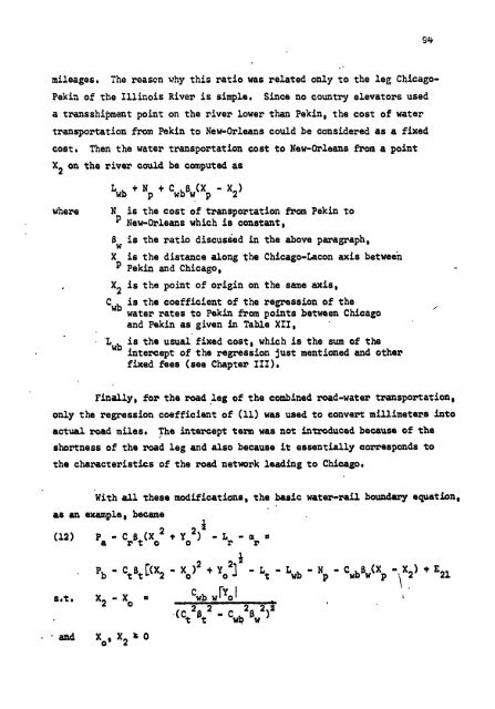
- Page 423 and 424: Table XIII. Boundary Equations. Wat
- Page 425 and 426: DIAGRAM 21 Figure T shows the actua
- Page 427 and 428: truck sample is small ( 148 origins
- Page 429 and 430: In this application of the spatial
- Page 431 and 432: NORTHWESTERN UNIVERSITY LIBRARY Man
- Page 433 and 434: in the dissertation. In addition, h
- Page 435 and 436: Analysis of Tow in Motion 66 Introd
- Page 437 and 438: Table • TABLES Statistical Result
- Page 439 and 440: deepening or widening the channel,
- Page 441 and 442: lines and isoquants. This locus is
- Page 443 and 444: limited to the cost and production
- Page 445 and 446: problem because engineers also atte
- Page 447 and 448: are ignored. Making sure that the r
- Page 449 and 450: variables, the form of the basic re
- Page 451 and 452: family of cost curves obtained in t
- Page 453 and 454: economies of scale exist in ihe tra
- Page 455 and 456: in which R = resistance, in taw-rop
- Page 457 and 458: (2)marginal productivity of the boa
- Page 459 and 460: conditions are not always met in pr
- Page 461 and 462: production relationship, e.g., a ma
- Page 463 and 464: Howe's production and planning mode
- Page 465 and 466: of the barge coefficient seemed to
- Page 467 and 468: 1962 counterparts. However, only (1
- Page 469 and 470: A 10 peicont increase in all inputs
- Page 471 and 472:
proportion of constant costs. Typic
- Page 473 and 474:
In short, cost was estimated as a f
- Page 475 and 476:
o f cars, etc.). Each is then multi
- Page 477 and 478:
haul. The variable (Z/X) was used i
- Page 479 and 480:
In the switching process--which con
- Page 481 and 482:
defined to be the percentage change
- Page 483 and 484:
other production analysis of rail i
- Page 485 and 486:
of transportation, the inputs contr
- Page 487 and 488:
It will be convenient to define T f
- Page 489 and 490:
vchicles, is considered to be a poi
- Page 491 and 492:
F t (v) = B/v. 6 Therefore, the equ
- Page 493 and 494:
The graphical expression of Equatio
- Page 495 and 496:
And the distance traveled, D c , du
- Page 497 and 498:
CHAPTER IV LINEHAUL PROCESS FUNCTIO
- Page 499 and 500:
Form of Process Function The proces
- Page 501 and 502:
particular . trip', that tonnage ma
- Page 503 and 504:
ostimated from a capacity cable for
- Page 505 and 506:
The function was originaliy fit by
- Page 507 and 508:
were greater than 11 miles per hour
- Page 509 and 510:
effective-push functions will be ex
- Page 511 and 512:
ilotilla. These assumptions will no
- Page 513 and 514:
Upon testing the hypotheses indicat
- Page 515 and 516:
for in the first case tows were sem
- Page 517 and 518:
a 0 / V I HP 3000 - 12 - 225 • H
- Page 519 and 520:
3.5 3.0 1.5 5.. 2.0 7, 4.0 ■•
- Page 521 and 522:
A final note concerning the effect
- Page 523 and 524:
predict the time required for trave
- Page 525 and 526:
Given the tonnage, 0, to be carried
- Page 527 and 528:
existence. For example, the locks o
- Page 529 and 530:
If all locks on the waterway arc tr
- Page 531 and 532:
loaded ones in 1950; therefore p is
- Page 533 and 534:
T L -2; Single Double Locking Locki
- Page 535 and 536:
u T L 1 Table 4.7 INDIVIDUAL AND SY
- Page 537 and 538:
it would leave the system. Alternat
- Page 539 and 540:
The government should incur the cos
- Page 541 and 542:
I si,:e was 3.1 bares. The small av
- Page 543 and 544:
To simplify the analysis all delay-
- Page 545 and 546:
characteristics and delays. Therefo
- Page 547 and 548:
Equation (4.37) divides the total :
- Page 549 and 550:
Xore confidence may be attached to
- Page 551 and 552:
Recapitulation of Tow Linehaul Proc
- Page 553 and 554:
function. The difference beiween th
- Page 555 and 556:
S -, speed of water, in miles per h
- Page 557 and 558:
y the above analysis, but for more
- Page 559 and 560:
econoinic analysis of the rail linc
- Page 561 and 562:
deceleration, Equation (3.8). Moreo
- Page 563 and 564:
Then the cargo weight of the ith ca
- Page 565 and 566:
(4, 6, or 8), the weight of the loc
- Page 567 and 568:
Analysis of Train in Motion Introdu
- Page 569 and 570:
and F(v) = 1.3w c + 29a 0.045w c v
- Page 571 and 572:
Adiustment for Grade and Curvature.
- Page 573 and 574:
Curve resistance, like grade resist
- Page 575 and 576:
F . 0 VI Fd(v) F (v) t Fig. 5.1 --
- Page 577 and 578:
and (5.26), and 2-miles-per-hour sp
- Page 579 and 580:
per trip into several components, e
- Page 581 and 582:
N t = number of trains on a given r
- Page 583 and 584:
Table 5.1 STATISTICAL ANALYSIS OF T
- Page 585 and 586:
Each of the terms V f and C represe
- Page 587 and 588:
nowever, in the case of the rail li
- Page 589 and 590:
-, 1 9, D 0 ,- ._ 200 ! i 175 '—
- Page 591 and 592:
Horsepowe r ( in t hou sa n ds ) 3
- Page 593 and 594:
exceeded 6,000 horsepower, for at p
- Page 595 and 596:
Curvatures of greater than 5 degree
- Page 597 and 598:
hohavior of rail costs. First, the
- Page 599 and 600:
eing charged at the higher rate. Th
- Page 601 and 602:
2. If train speed is greater than o
- Page 603 and 604:
maximula attainable horsepower of t
- Page 605 and 606:
price for each locomotive unit from
- Page 607 and 608:
I L' is given by (0.5)($94HP L - $4
- Page 609 and 610:
Figure 5.4 displays a set of short-
- Page 611 and 612:
Economics of scale, in fact, seem t
- Page 613 and 614:
Tab1e 5.8 LONG-RUN MARGINAL COST OF
- Page 615 and 616:
obtained this way may then be added
- Page 617 and 618:
The estimating methods for each of
- Page 619 and 620:
Cos t per ton -mi le (m ;1 1s ) 7.2
- Page 621 and 622:
CHAPTER VI SUMMARY AND CONCLUSIONS
- Page 623 and 624:
eached for acceleration, which take
- Page 625 and 626:
wide range of output would have to
- Page 627 and 628:
Isoquants between car and locomotiv
- Page 629 and 630:
eported in the dissertation will in
- Page 631 and 632:
10. M. Bronfenbrenner and P. H. Dou
- Page 633 and 634:
13. A. V.ctor Cabot and Arthur P. H
- Page 635 and 636:
7. There are in fact three differen
- Page 637 and 638:
26. Eric Bottoms, "Practical Tonnag
- Page 639 and 640:
19. Hay, An Introduction to Transpo
- Page 641 and 642:
BIBLIOGRAPHY American Railway Engin
- Page 643 and 644:
Howe, Charles M... "Methods for Equ
- Page 645 and 646:
Soberman, Richard. "A Railway Perfo
- Page 647 and 648:
NORTHWESTERN UNIVERSITY ESTIMATION
- Page 649 and 650:
TABLE OF COIMETS Page Chapter I. In
- Page 651 and 652:
CHAPTER I INTRODUCTION AND REVIEW O
- Page 653 and 654:
On the other hand, the statistical
- Page 655 and 656:
and capital Outlays are also treate
- Page 657 and 658:
TABLE 1 SUMMARY ESTIMATES OF RAILRO
- Page 659 and 660:
C (X) FIGURE • ■ 9
- Page 661 and 662:
The effects of two types of classif
- Page 663 and 664:
egression equations will produce bi
- Page 665 and 666:
S = speed in miles per hour W = wid
- Page 667 and 668:
(6) S = h(HP, L, B, H, D, W) The ac
- Page 669 and 670:
stock which remains idle. Under the
- Page 671 and 672:
The planning function also exhibite
- Page 673 and 674:
Of the production functions, (13, 1
- Page 675 and 676:
sources of data. Despite the use of
- Page 677 and 678:
The reader should note several them
- Page 679 and 680:
from variations in rates based on v
- Page 681 and 682:
service the firm would want to set
- Page 683 and 684:
oat output, or effort, is not propo
- Page 685 and 686:
this level of disaggregation are ex
- Page 687 and 688:
CHAPTER III A STATISTICAL PRODUCTIO
- Page 689 and 690:
A second way of generating data inv
- Page 691 and 692:
variables, even if it is not accura
- Page 693 and 694:
Three major inland waterway firms p
- Page 695 and 696:
from changing depth or stream flow.
- Page 697 and 698:
made for each. (In the log-linear r
- Page 699 and 700:
•Ps Variable Name Riven Districts
- Page 701 and 702:
Variable Name River Districts Port
- Page 703 and 704:
La Variable Name River Districts TA
- Page 705 and 706:
Variable Name River Districts TABLE
- Page 707 and 708:
t..n .....1 TABLE 6 . . VARIABLE ME
- Page 709 and 710:
A. Linear Regression (Arithi.etic M
- Page 711 and 712:
are roughly comparable across all c
- Page 713 and 714:
termed "labor embodied technologica
- Page 715 and 716:
TABLE 8 COMPANY ONE LINEAR REGRESSI
- Page 717 and 718:
the other monthly coefficients indi
- Page 719 and 720:
CHAPTER IV AN ANALYSIS OF DIRECT TO
- Page 721 and 722:
with the use of dummy variables. To
- Page 723 and 724:
A more direct method, and the one e
- Page 725 and 726:
. cost In using; for example, , cro
- Page 727 and 728:
• ,,, • .. -Excluded Variables
- Page 729 and 730:
200,000 EBM per year) comes to abou
- Page 731 and 732:
Form C weights have limited accurac
- Page 733 and 734:
study as to the level of output to
- Page 735 and 736:
The firm in the sample operates a l
- Page 737 and 738:
would tend to be slightly higher co
- Page 739 and 740:
3. other bulk 4. petroleum products
- Page 741 and 742:
In addition, river districts with s
- Page 743 and 744:
where: Cost = annual total direct b
- Page 745 and 746:
1964 1965 Variable Name Barge Type
- Page 747 and 748:
TABLE 13 F-TESTS FOR BARGE COST REG
- Page 749 and 750:
tend to rise with increases in barg
- Page 751 and 752:
ing is quite consistent with a prio
- Page 753 and 754:
TABLE 16 PERCENT COMMODITY REGRESSI
- Page 755 and 756:
arge was to ship one more commodity
- Page 757 and 758:
1 are the costs of operating and ma
- Page 759 and 760:
preparation of barges is necessary
- Page 761 and 762:
estimated was the same for all thre
- Page 763 and 764:
TABLE 17 DIRECT BARGE EXPENSE r 2 =
- Page 765 and 766:
Variable Name TABLE 19 TERMINAL EXP
- Page 767 and 768:
considerable growth in the past twe
- Page 769 and 770:
also be used in conjunction with di
- Page 771 and 772:
to an already scheduled tow). Two k
- Page 773 and 774:
The terminal results are quite tent
- Page 775 and 776:
The five firms in the sample repres
- Page 777 and 778:
sure the extent of this activity, a
- Page 779 and 780:
1 linear form of- the functions hav
- Page 781 and 782:
C. Net Tons of Barge Capacity TABLE
- Page 783 and 784:
Indirect cost is the same for towbo
- Page 785 and 786:
A. Total Horsepower TABLE 22 CROSS
- Page 787 and 788:
1 .‘ A. Total Horsepower TABLE 23
- Page 789 and 790:
to scheduling. In addition, we obse
- Page 791 and 792:
:CHAPTER VII SUMMARY AND CONCLUSION
- Page 793 and 794:
the coefficients of the dummy varia
- Page 795 and 796:
. The coefficients of the dummy var
- Page 797 and 798:
Supporting results for neutral tech
- Page 799 and 800:
port agencies. A considerable amoun
- Page 801 and 802:
I to inland waterway operators, sin
- Page 803 and 804:
Footnotes--Continued 7 Howe, Jan.,
- Page 805 and 806:
Footnotes--Continued This is also w
- Page 807 and 808:
Bibliography--Continued Interstate
- Page 809 and 810:
UNCLASSIFIED Security Classificatio