

Mathematics in Independent Component Analysis
Mathematics in Independent Component Analysis
Mathematics in Independent Component Analysis

Create successful ePaper yourself
Turn your PDF publications into a flip-book with our unique Google optimized e-Paper software.
106 Chapter 5. IEICE TF E87-A(9):2355-2363, 2004<br />
THEIS and NAKAMURA: QUADRATIC INDEPENDENT COMPONENT ANALYSIS<br />
yi = b ⊤ i s. (5)<br />
We will show that we can assume B to be <strong>in</strong>vertible.<br />
If B is not <strong>in</strong>vertible, without loss of generality let<br />
bn = �n−1 i=1 λibi with coefficients λi ∈ R. Then at least<br />
one λi �= 0, otherwise yn = 0 is determ<strong>in</strong>istic. Without<br />
loss of generality let λ1 = 1. From equation 5 we then<br />
get yn = �n−1 i=1 λiyi = y1+u with u := �n−1 i=2 λiyi <strong>in</strong>dependent<br />
of y1. Application of the Darmois-Skitovitch<br />
theorem [6, 16] to the two equations<br />
y1 = y1<br />
yn = y1 + u<br />
shows that y1 is Gaussian or determ<strong>in</strong>istic. Hence all<br />
yi with λi �= 0 are Gaussian or determ<strong>in</strong>istic. So we<br />
may assume that y1, yn and u are square <strong>in</strong>tegrable.<br />
Without loss of generality let those random variables<br />
be centered. Then the cross-covariance of (y1, yn) can<br />
be calculated as follows:<br />
0 = E(y1y ⊤ n ) = E(y1y ⊤ 1 ) + E(y1u ⊤ ) = var y1,<br />
so y1 is determ<strong>in</strong>istic. Hence all yi with λi �= 0 are<br />
determ<strong>in</strong>istic, and then also yn. So at least two components<br />
of y = Wx are determ<strong>in</strong>istic <strong>in</strong> contradiction<br />
to the assumption. Therefore B is <strong>in</strong>vertible.<br />
Us<strong>in</strong>g assumptions i) or ii) and the well-known<br />
uniqueness result of square l<strong>in</strong>ear BSS — a corollary<br />
[5, 7] of the Darmois-Skitovitch theorem, see [17] for a<br />
proof without us<strong>in</strong>g this theorem — there exist a permutation<br />
matrix P and an <strong>in</strong>vertible scal<strong>in</strong>g matrix L<br />
with WA = LP. The properties of the pseudo <strong>in</strong>verse<br />
then show that the equation<br />
(LP) −1 WA = I<br />
<strong>in</strong> W has solutions W = LP(A + + C ′ ) with C ′ A = 0,<br />
or W = LPA + + C aga<strong>in</strong> with CA = 0.<br />
The pseudo <strong>in</strong>verse is the unique solution of WA =<br />
I with m<strong>in</strong>imum Frobenius norm. In this case C = 0;<br />
so if W is an ICA of x with m<strong>in</strong>imal Frobenius norm,<br />
then already W equals A + except for scal<strong>in</strong>g and permutation.<br />
This can be used for normalization. Us<strong>in</strong>g<br />
s<strong>in</strong>gular value decomposition of A, this has been shown<br />
and extended to the noisy case <strong>in</strong> [14].<br />
Theorem 2.1 states that <strong>in</strong> the case where x is the<br />
mixture of n sources,<br />
s<br />
A<br />
.. x<br />
W<br />
W ′<br />
. .<br />
. .<br />
y<br />
.................... .<br />
y ′<br />
W ′ A<br />
ignor<strong>in</strong>g the always present scal<strong>in</strong>g and permutation<br />
(then y = y ′ = s), we have an n(m − n)-dimensional<br />
aff<strong>in</strong>e vector space as ICAs of x i.e. (W − W ′ )A = 0.<br />
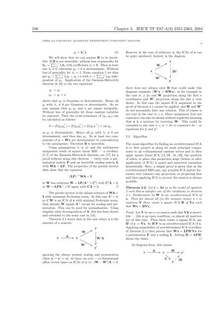
However <strong>in</strong> the case of arbitrary x, the ICAs of x can<br />
be quite unrelated. Indeed, <strong>in</strong> the diagram<br />
x<br />
W<br />
W ′<br />
..<br />
. .<br />
y<br />
...<br />
..<br />
..<br />
...<br />
. .<br />
y ′<br />
∃B?<br />
there does not always exist B that could make this<br />
diagram commute (W ′ x = BWx), as for example <strong>in</strong><br />
the case m ≥ 2n and W projection along the first n<br />
coord<strong>in</strong>ates and W ′ projection along the last n ones<br />
shows. In this case the square ICA argument <strong>in</strong> the<br />
proof of theorem 2.1 cannot be applied, and W and W ′<br />
do not necessarily have any relation. This of course is<br />
not true <strong>in</strong> the case m = n, where uniqueness (but not<br />
existence) can also be shown without explicitly know<strong>in</strong>g<br />
that x is a mixture by <strong>in</strong>vert<strong>in</strong>g W. This could be<br />
extended to the case n ≤ m < 2n to construct 2n − m<br />
equations for y and y ′ .<br />
2.3 Algorithm<br />
The usual algorithm for f<strong>in</strong>d<strong>in</strong>g an overdeterm<strong>in</strong>ed ICA<br />
is to first project x along its ma<strong>in</strong> pr<strong>in</strong>cipal components<br />
to an n-dimensional random vector and to then<br />
apply square l<strong>in</strong>ear ICA [14, 19]. In [19], the question<br />
of where to place this projection stage (before or after<br />
application of ICA) is posed and answered somewhat<br />
heuristically. Here, a simple proof is given that <strong>in</strong> the<br />
overdeterm<strong>in</strong>ed BSS case, any possible ICA matrix factorizes<br />
over (almost) any projection, so project<strong>in</strong>g first<br />
and then apply<strong>in</strong>g ICA to recover the sources is always<br />
possible.<br />
Theorem 2.2. Let x = As as <strong>in</strong> the model of equation<br />
2 such that s satisfies one of the conditions <strong>in</strong> theorem<br />
2.1. Furthermore let W be an overdeterm<strong>in</strong>ed ICA of<br />
x. Then for almost all (<strong>in</strong> the measure sense) n × m<br />
matrices V there exists a square ICA B of Vx such<br />
that Wx = BVx.<br />
Proof. Let V be an n×m matrix such that VA is <strong>in</strong>vertible<br />
— this is an open condition, so almost all matrices<br />
are of this type. Then there exists a square ICA, say<br />
B ′ of y := Vx. So B ′ V is an overdeterm<strong>in</strong>ed ICA of x.<br />
Apply<strong>in</strong>g separability of overdeterm<strong>in</strong>ed ICA (corollary<br />
of theorem 2.1) then proves that Wx = LPB ′ Vx for<br />
a permutation P and a scal<strong>in</strong>g L. Sett<strong>in</strong>g B := LPB ′<br />
shows the claim.<br />
In diagram-form, this means<br />
A . .<br />
s x y ′ W<br />
..<br />
V<br />
. ..<br />
y<br />
. . ..<br />
∃B<br />
3


