Mathematics in Independent Component Analysis

Chapter 11. EURASIP JASP, 2007 165
4 EURASIP Journal on Advances in Signal Processing
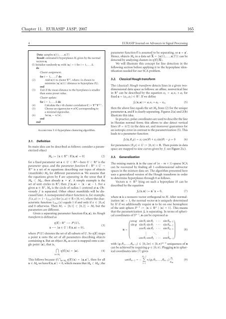
Data: samples x(1), . . . , x(T)
Result: estimated k hyperplanes Hi given by the normal
vectors ui
(l) Initialize randomly ui with |ui| = 1 for i = 1, . . . , k.
do
Cluster assignment.
for t ← 1, . . . , T do
(2) Add x(t) to cluster Y (i) , where i is chosen to
minimize |u ⊤ i x(t)| (distance to hyperplane Hi).
end
(3) Exit if the mean distance to the hyerplanes is smaller
than some preset value.
Cluster update.
for i ← 1, . . . , k do
(4) Calculate the i-th cluster correlation C := Y (i) Y (i)⊤ .
(5) Choose an eigenvector v of C corresponding to
a minimal eigenvalue.
(6) Set ui ← v/|v|.
end
end
Algorithm 3: k-hyperplane clustering algorithm.
3.1. Definition
Its main idea can be described as follows: consider a parameterized
object
Ma := {x ∈ R n | f(x, a) = 0} (2)
for a fixed parameter set a ∈ U ⊂ R p —here U ⊂ R p is the
parameter space, and the parameter function f : R n × U →
R m is a set of m equations describing our types of objects
(manifolds) Ma for different parameters a. We assume that
the equations given by f are separating in the sense that if
Ma ⊂ Ma ′, then already a = a′ . A simple example is the
set of unit circles in R 2 ; then f (x, a) = |x − a| − 1. For a
given a ∈ R 2 , Ma is the circle of radius 1 centered at a. Obviously
f is separated. Other object manifolds will be discussed
later. A nonseparated object function is, for example,
f (x, a) := 1−1[0,a](x) for (x, a) ∈ R×[0, ∞), where the characteristic
function 1[0,a](x) equals 1 if and only if x ∈ [0, a]
and 0 otherwise. Then M1 = [0, 1] ⊂ [0, 2] = M2 but the
parameters are different.
Given a separating parameter function f(x, a), its Hough
transform is defined as
η[f] : R n −→ P (U),
x ↦−→ {a ∈ U | f(x, a) = 0},
where P (U) denotes the set of all subsets of U. So η[f] maps
a point x onto the set of all parameters describing objects
containing x. But an object Ma as a set is mapped onto a single
point {a}, that is,
�
η[f](x) = {a}. (4)
x∈Ma
This follows because if �
x∈Ma η[f](x) = {a, a′ }, then for all
x ∈ Ma we have f(x, a ′ ) = 0, which means that Ma ⊂ Ma ′; the
(3)
parameter function f is assumed to be separating, so a = a ′ .
Hence, objects Ma in a data set X = {x(1), . . . , x(T)} can be
detected by analyzing clusters in η[f](X).
We will illustrate this concept for line detection in the
following section before applying it to the hyperplane identification
needed for our SCA problem.
3.2. Classical Hough transform
The (classical) Hough transform detects lines in a given twodimensional
data space as follows: an affine, nonvertical line
in R 2 can be described by the equation x2 = a1x1 + a2 for
fixed a = (a1, a2) ∈ R 2 . If we define
fL(x, a) := a1x1 + a2 − x2, (5)
then the above line equals the set Ma from (2) for the unique
parameter a, and f is clearly separating. Figures 2(a) and 2(b)
illustrate this idea.
In practice, polar coordinates are used to describe the line
in Hessian normal form; this allows to also detect vertical
lines (θ = π/2) in the data set, and moreover guarantees for
an isotropic error in contrast to the parametrization (5). This
leads to a parameter function
fP(x, θ, ρ) = x1 cos(θ) + x2 sin(θ) − ρ = 0 (6)
for parameters (θ, ρ) ∈ U := [0, π) × R. Then points in data
space are mapped to sine curves given by f ; see Figure 2(c).
3.3. Generalization
The mixing matrix A in the case of (n − m + 1)-sparse SCA
can be recovered by finding all 1-codimensional subvector
spaces in the mixture data set. The algorithm presented here
uses a generalized version of the Hough transform in order
to determine hyperplanes through 0 as follows.
Vectors x ∈ R m lying on such a hyperplane H can be
described by the equation
fh(x, n) := n ⊤ x = 0, (7)
where n is a nonzero vector orthogonal to H. After normalization
|n| = 1, the normal vector n is uniquely determined
by H if we additionally require n to lie on one hemisphere
of the unit sphere Sn−1 := {x ∈ Rn | |x| = 1}. This means
that the parametrization fh is separating. In terms of spherical
coordinates of Sn−1 , n can be expressed as
⎛
⎞
cos ϕ sin θ1 sin θ2 · · · sin θm−2
⎜
⎜sin
ϕ sin θ1 sin θ2 · · · sin θm−2
⎟
⎜
n = ⎜ cos θ1 sin θ2 · · · sin ⎟
θm−2⎟
⎜ . .
⎝ . ..
.
⎟ (8)
⎟
. ⎠
cos θ1 cos θ2 · · · cos θm−2
with (ϕ, θ1, . . . , θm−2) ∈ [0, 2π) × [0, π) m−2 uniqueness of n
can be achieved by requiring ϕ ∈ [0, π). Plugging n in spherical
coordinates into (7) gives
m−1 �
cot θm−2 = − νi(ϕ, θ1, . . . , θm−3) xi
i=1
xm
(9)