Mathematics in Independent Component Analysis

194 Chapter 14. Proc. ICASSP 2006
Algorithm 2: Projection onto S n−1
p via fixed-point iteration.
Again, the iteration is to be stopped after only sufficiently small
updates are taken.
Input: vector x∈R n
Output: Euclidean projection y=π S n−1 (x)
p
Initialize y∈S n−1
1
p randomly.
for i←1, 2,... do
λ← �n i=1 (yi−xi)/ � n sgn(yi)|yi| p−1�
2
y←x+λ sgn(y)|y| ⊙(p−1)
3
4 y←y/�y�p
end
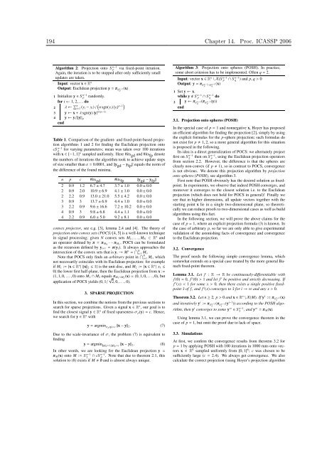
Table 1. Comparison of the gradient- and fixed-point-based projection
algorithms 1 and 2 for finding the Euclidean projection onto
cS n−1
p for varying parameters; mean was taken over 100 iterations
with x∈[−1, 1] n sampled uniformly. Here #itsgd and #itsfp denote
the numbers of iterations the algorithm took to achieve update steps
of size smaller thanε=0.0001, and�y gd− yfp� equals the norm of
the difference of the found minima.
n p c #its gd #its fp �y gd − y fp �
2 0.9 1.2 6.7±4.7 3.7±1.0 0.0±0.0
2 0.9 2.0 10.9±6.9 4.1±1.0 0.0±0.0
2 2.2 0.9 13.0±21.0 5.5±4.2 0.0±0.0
3 0.9 3 13.7±6.9 4.4±1.0 0.0±0.0
3 2.2 0.9 9.6±16.6 7.2±10.2 0.0±0.0
4 0.9 3 9.8±6.8 4.4±1.1 0.0±0.0
4 2.2 0.9 6.0±5.0 9.2±8.1 0.0±0.0
convex projector, see e.g. [3], lemma 2.4 and [4]. The theory of
projection onto convex sets (POCS) [4, 5] is a well-known technique
in signal processing; given N convex sets M1,..., MN ⊂ R n and
an operator defined byπ=πMN ···πM1 , POCS can be formulated
as the recursion defined by yi+1=π(yi). It always approaches the
intersection of the convex sets that is yi→M ∗ = �N i=1 Mi.
Note that POCS only finds an arbitrary point in �N i=1 Mi, which
not necessarily coincides with its Euclidean projection: for example
if M1 :={x∈R n |�x�2≤ 1} is the unit disc, and M2 :={x∈R n | x1≤
0} the lower first half-plane, then the Euclidean projection from x :=
(1, 1, 0,...,0) onto M1∩M2 equalsπM1∩M2 (x)=(0, 1, 0,...,0), but
application of POCS yields (0, 1/ √ 2, 0,...,0).
3. SPARSE PROJECTION
In this section, we combine the notions from the previous sections to
search for sparse projections. Given a signal x∈R n , our goal is to
find the closest signal y∈R n of fixed sparsenessσp(y)=c. Hence,
we search for y∈R n with
y=argmin σp(y)=c �x−y�2. (7)
Due to the scale-invariance ofσ, the problem (7) is equivalent to
finding
y=argmin �y�2=1,�y�p=c �x−y�2. (8)
In other words, we are looking for the Euclidean projection y =
πM(x) onto M := S n−1 n−1
2 ∩ cS p . Note that due to theorem 2.1, this
solution to (8) exists if M�∅ and is almost always unique.
Algorithm 3: Projection onto spheres (POSH). In practice,
some abort criterion has to be implemented. Often q=2.
Input: vector x∈R n \X(S n−1
p ∩ S n−1
q ) and p, q>0
Output: y=π S n−1 (x)
p ∩S n−1
q
1 Set y←x.
while y�S n−1
p ∩ S n−1
q do
2 y←π S n−1 (π
q S n−1 (y))
p
end
3.1. Projection onto spheres (POSH)
In the special case of p=1 and nonnegative x, Hoyer has proposed
an efficient algorithm for finding the projection [2], simply by using
the explicit formulas for the p-sphere projection; such formulas do
not exist for p�1, 2, so a more general algorithm for this situation
is proposed in the following.
Its idea is a direct generalization of POCS: we alternately project
first on S n−1 then on S n−1
p , using the Euclidean projection operators
2
from section 2.2. However, the difference is that the spheres are
clearly non-convex (if p�1), so in contrast to POCS, convergence
is not obvious. We denote this projection algorithm by projection
onto spheres (POSH), see algorithm 3.
First note that POSH obviously has the desired solution as fixedpoint.
In experiments, we observe that indeed POSH converges, and
moreover it converges to the closest solution i.e. to the Euclidean
projection (which does not hold for POCS in general)! Finally we
see that in higher dimensions, all update vectors together with the
starting point x lie in a single two-dimensional plane, so theoretically
we can reduce proofs to two-dimensional cases as well as build
algorithms using this fact.
In the following section, we will prove the above claims for the
case of p=1, where an explicit projection formula (3) is known. In
the case of arbitrary p, so far we are only able to give experimental
validation of the astonishing facts of convergence and convergence
to the Euclidean projection.
3.2. Convergence
The proof needs the following simple convergence lemma, which
somewhat extends on a special case treated by the more general Banach
fixed-point theorem.
Lemma 3.1. Let f : R→R be continuously-differentiable with
f (0)=0, f ′ (0)>1 and let f ′ be positive and strictly decreasing. If
f ′ (x)0, then there exists a single positive fixedpoint
ˆx of f , and f i (x) converges to ˆx for i→∞ and any x>0.
Theorem 3.2. Let n≥2, p>0 and x∈R n \X(M). If y1 :=π S n−1 (x)
2
and iteratively y i :=π S n−1
2
(π S n−1
1
(y i−1 )) according to the POSH algo-
rithm, then y i converges to some y ∞ ∈ S n−1
2 , and y ∞ =πM(x).
Using lemma 3.1, we can prove the convergence theorem in the
case of p=1, but omit the proof due to lack of space.
3.3. Simulations
At first, we confirm the convergence results from theorem 3.2 for
p=1by applying POSH with 100 iterations in 1000 runs onto vectors
x ∈ R 6 sampled uniformly from [0, 1] 6 ; c was chosen to be
sufficiently large (c=2.4). We always get convergence. We also
calculate the correct projection (using Hoyer’s projection algorithm