Mathematics in Independent Component Analysis

Chapter 13. Proc. EUSIPCO 2005 187
M X (M)
(a) exception set of two points
M
X (M)
(b) exception set of a sector
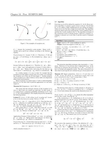
Figure 1: Two examples of exception sets.
if 〈.,.〉 denotes the (symmetric) scalar product. Hence 〈a,b〉 =
�a��b� and a and b are collinear according to the Schwarz inequality.
Proof of lemma 2.4. Assume X (M) �= ∅. Then let x ∈ X (M) and
p1 �= p2 ∈ M such that pi ⊳x. By assumption q := 1 2 (p1 +p2) ∈
M. But
�x −p1� ≤ �x −q� ≤ 1
1
�x −p1�+
2 2 �x −p2� = �x −p1�
because both pi are adjacent to x. Therefore �x −q� = � 1 2 (x −
p1)�+� 1 2 (x −p2)� and application of lemma 2.5 shows that x −
p1 = α(x −p2). Taking norms (and using the fact that q �= x)
shows that α = 1 and hence p1 = p2, which is a contradiction.
In a similar manner, it is easy to show for example that the
exception set of the sphere consists only of its center, or to calculate
the exception sets of the sets M from figure 1. Another property
of the exception set is that it behaves nicely under non-degenerate
affine linear transformation.
Hence in general, we cannot expect X (M) to vanish altogether.
However we can show that in practical applications we can easily
neglect it:
Theorem 2.6 (Uniqueness). vol(X (M)) = 0.
This means that the Lebesgue measure of the exception set is
zero i.e. that it does not contain any open ball. In other words, if
x is drawn from a continuous probability distribution on R n , then
x ∈X (M) with probability 0. We simplify the proof by introducing
the following lemma:
Lemma 2.7. Letx∈X (M) withp⊳x,p ′ ⊳x and p �=p ′ . Assume
y lies on the line between x and p. Then y �∈ X (M).
Proof. So y = αx+(1 − α)p with α ∈ (0,1). Note that then also
p⊳y — otherwise we would have another q⊳y with �q −y� <
�p−y�. But then �q−x� ≤ �q−y�+�y−x� < �p−y�+�y−
x� = �p −x�, which contradicts the assumption.
Now assume that y ∈ X (M). Then there exists p ′′ ⊳y with
p ′′ �= p. But �p ′′ −x� ≤ �p ′′ −y�+�y −x� = �p −y�+�y −
x� = �p −x�. Then p⊳x induces �p ′′ −x� = �p −x�. So
�p ′′ −x� = �p ′′ −y�+�y −x�.
Application of lemma 2.5 then yields p ′′ −y = α(y−x), and hence
p ′′ −y = β(p −y). Taking norms (and using p ⊳x) shows that
β = 1 and hence p = p ′′ , which is a contradiction.
Proof of theorem 2.6. Assume there exists an open set U ⊂ X (M),
and let x ∈ U. Then choose p �= p ′ ∈ M with p⊳x,p ′ ⊳x. But
{αx+(1 − αp)|α ∈ (0,1)} ∩U �= ∅,
which contradicts lemma 2.7.
2.3 Algorithm
From here on, let M be defined by equation (2). In [2], Hoyer proposes
algorithm 1 to project a given vector x onto p ∈ M such that
p⊳x (we added a slight simplification by not setting all negative
values of s to zero but only a single one in each step). The algorithm
iteratively detects p by first satisfying the 1-norm condition (line 1)
and then the 2-norm condition (line 3). The algorithm terminates if
the constructed vector is already positive; otherwise a negative coordinate
is selected, set to zero (line 4) and the search is continued
in R n−1 .
Algorithm 1: Sparse projection
Input: vector x ∈ R n , norm conditions λ1 and λ2
Output: closest non-negative s with �s�i = λi
Set r ← x+(�x�1 − λ1/n)e with e = (1,...,1) ⊤ ∈ Rn 1
.
2 Set m ← (λ1/n)e.
3 Set s ← m+α(r −m) with α > 0 such that �s�2 = λ2.
if exists j with s j < 0 then
4 Fix s j ← 0.
5 Remove j-th coordinate of x.
6 Decrease dimension n ← n − 1.
7 goto 1.
end
The projection algorithm terminates after maximally n − 1 iterations.
However it is not obvious that it indeed detects p. In the
following we will prove this given that x �∈ X (M) — of course we
have to exclude non-uniqueness points. The idea of the proof is to
show that in each step the new estimate has p as closest point in M.
Theorem 2.8 (Sparse projection). Given x ≥ 0 such that x �∈
X (M). Let p ∈ M with p ⊳ x. Furthermore assume that r and
s are constructed by lines 1 and 3 of algorithm 1. Then:
(i) ∑ri = λ1, p⊳r and r �∈ X (M).
(ii) ∑si = λ1, �s�2 = λ2 and p⊳s and s �∈ X (M).
(iii) If s j < 0 then p j = 0.
(iv) Define u := s but set u j = 0. Then p⊳u and u �∈ X (M).
This theorem shows that if s ≥ 0 then already s ∈ M and p⊳s
(ii) so s = p. If s j < 0 then it is enough to set s j := 0 (because
p j = 0 (iii)) and continue the search in one dimension lower (iv).
Proof. Let H := {x ∈ R n |∑xi = λ1} denote the affine hyperplane
given by the 1-norm. Note that M ⊂ H.
(i) By construction r ∈ H. Furthermore e⊥H, so r is the orthogonal
projection of x onto H. Let q ∈ M be arbitrary. We then
get �q−x� 2 = �q−r� 2 +�r−x� 2 . By definition �p−x� ≤ �q−
x�, so �p −r� 2 = �p −x� 2 − �r −x� 2 ≤ �q −x� 2 − �r −x� 2 =
�q −r� 2 and therefore p⊳r. Furthermore r �∈ X (M) because if
q ∈ R n with q⊳r, then �q−r� = �p−r�. Then by the above also
�q −x� = �p −x�, hence q = p (because x �∈ X (M)).
(ii) First note that s is a linear combination of m and r, and both
lie in H so also s ∈ H i.e. ∑si = λ1. Furthermore by construction
�s� = λ2. Now let q ∈ M. For p⊳s to hold, we have to show that
�p −s� ≤ �q −s�. This follows (see (i)) if we can show
�q −r� 2 = �s −r� 2 + 1
�q −s�
α0
2 . (3)
We can prove this equation as follows: By definition λ 2 2 = �q −
m�2 = �q −s�2 + �s −m�2 + 2〈q −s,s −m〉, hence �q −s�2 =
−2〈q−s,s−m〉 = −2 α0
α0−1 〈q−s,s−r〉, where we have used s−
m = α0(r −m) i.e. m = s−α0r
1−α0
α0
so s −m = α0−1 (s −r).