Mathematics in Independent Component Analysis

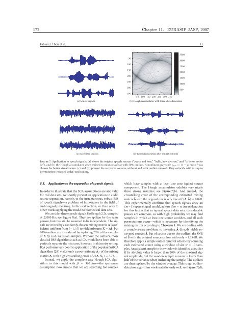
172 Chapter 11. EURASIP JASP, 2007
Fabian J. Theis et al. 11
(a) Source signals
50
100
150
200
250
300
350
50 100 150 200 250 300 350
(b) Hough accumulator with three labeled maxima
(c) Recovered sources (d) Recovered sources after outlier removal
Figure 7: Application to speech signals: (a) shows the original speech sources (“peace and love,” “hello, how are you,” and “to be or not to
be”), and (b) the Hough accumulator when trained to mixtures of (a) with 20% outliers. A nonlinear gray scale γnew := (1 − γ/ max) 10 was
chosen for better visualization. (c) and (d) present the recovered sources, without and with outlier removal. They coincide with (a) up to
permutation (reversed order) and scaling.
5.5. Application to the separation of speech signals
In order to illustrate that the SCA assumptions are also valid
for real data sets, we shortly present an application to audio
source separation, namely, to the instantaneous, robust BSS
of speech signals—a problem of importance in the field of
audio signal processing. In the next section, we then refer to
other works applying the model to biomedical data sets.
We consider three speech signals S of length 2.2s, sampled
at 22000 Hz; see Figure 7(a). They are spoken by the same
person, but may still be assumed to be independent. The signals
are mixed by a randomly chosen mixing matrix A (coefficients
uniform from [−1, 1]) to yield mixtures X = AS, but
20% outliers are introduced by replacing 20% of the samples
of X by i.i.d. Gaussian samples. Without the outliers, more
classical BSS algorithms such as ICA would have been able to
perfectly separate the mixtures; however, in this noisy setting,
ICA performs very poorly: application of the popular fastICA
algorithm [29] yields only a poor estimate �A f of the mixing
matrix A, with high crosstalking error of E(A, �A f ) = 3.73.
Instead, we apply the complete-case Hough-SCA algorithm
to this model with β = 360 bins—the sparseness
assumption now means that we are searching for sources,
3500
3000
2500
2000
1500
1000
which have samples with at least one zero (quiet) source
component. The Hough accumulator exhibits very nicely
three strong maxima; see Figure 7(b). And indeed, the
crosstalking error of the corresponding estimated mixing
matrix �A with the original one is very low at E(A, �A) = 0.020.
This experimentally confirms that speech signals obey an
(m−1)-sparse signal model, at least if m = n. An explanation
for this fact is that in typical speech data sets, considerable
pauses are common, so with high probability we may find
samples in which at least one source vanishes, and all such
permutations occur—which is necessary for identifying the
mixing matrix according to Theorem 1. We are dealing with
a complete-case problem, so inverting �A directly yields recovered
sources �S. But of course due to the outliers, the SNR
of �S with the original sources is low with only −1.35 dB. We
therefore apply a simple outlier removal scheme by scanning
each estimated source using a window of size w = 10 samples.
An adjacent sample to the window is identified as outlier
if its absolute value is larger than 20% of the maximal signal
amplitude, but the window sample variance is lower than
half of the variance when including the sample. The outliers
are then replaced by the window average. This rough outlierdetection
algorithm works satisfactorily well, see Figure 7(d);
500