Mathematics in Independent Component Analysis
Mathematics in Independent Component Analysis
Mathematics in Independent Component Analysis
Create successful ePaper yourself
Turn your PDF publications into a flip-book with our unique Google optimized e-Paper software.
Chapter 17. IEEE SPL 13(2):96-99, 2006 241<br />
IEEE SIGNAL PROCESSING LETTERS, VOL. X, NO. XX, XXXX 2<br />
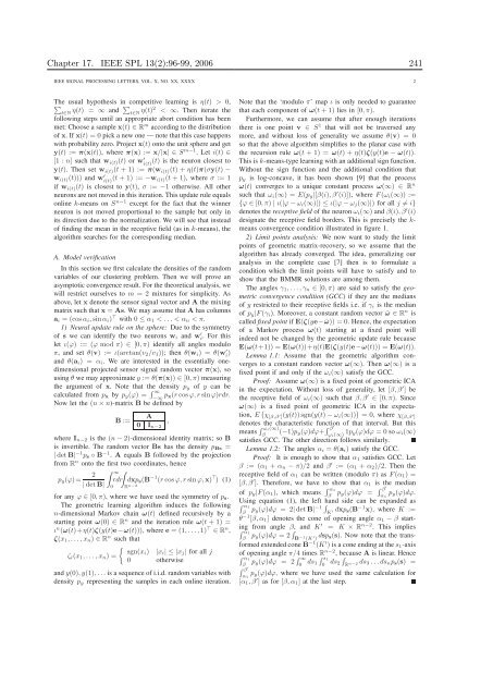
The<br />
�<br />
usual hypothesis <strong>in</strong><br />
�<br />
competitive learn<strong>in</strong>g is η(t) > 0,<br />
t∈N η(t) = ∞ and t∈N η(t)2 < ∞. Then iterate the<br />
follow<strong>in</strong>g steps until an appropriate abort condition has been<br />
met: Choose a sample x(t) ∈ Rm accord<strong>in</strong>g to the distribution<br />
of x. If x(t) = 0 pick a new one — note that this case happens<br />
with probability zero. Project x(t) onto the unit sphere and get<br />
y(t) := π(x(t)), where π(x) := x/|x| ∈ Sm−1 . Let i(t) ∈<br />
[1 : n] such that wi(t)(t) or w ′ i(t) (t) is the neuron closest to<br />
y(t). Then set wi(t)(t + 1) := π(wi(t)(t) + η(t)π(σy(t) −<br />
wi(t)(t))) and w ′ i(t) (t + 1) := −wi(t)(t + 1), where σ := 1<br />
if wi(t)(t) is closest to y(t), σ := −1 otherwise. All other<br />
neurons are not moved <strong>in</strong> this iteration. This update rule equals<br />
onl<strong>in</strong>e k-means on Sn−1 except for the fact that the w<strong>in</strong>ner<br />
neuron is not moved proportional to the sample but only <strong>in</strong><br />
its direction due to the normalization. We will see that <strong>in</strong>stead<br />
of f<strong>in</strong>d<strong>in</strong>g the mean <strong>in</strong> the receptive field (as <strong>in</strong> k-means), the<br />
algorithm searches for the correspond<strong>in</strong>g median.<br />
A. Model verification<br />
In this section we first calculate the densities of the random<br />
variables of our cluster<strong>in</strong>g problem. Then we will prove an<br />
asymptotic convergence result. For the theoretical analysis, we<br />
will restrict ourselves to m = 2 mixtures for simplicity. As<br />
above, let x denote the sensor signal vector and A the mix<strong>in</strong>g<br />
matrix such that x = As. We may assume that A has columns<br />
ai = (cosαi, s<strong>in</strong>αi) ⊤ with 0 ≤ α1 < . . . < αn < π.<br />
1) Neural update rule on the sphere: Due to the symmetry<br />
of s we can identify the two neurons wi and w ′ i<br />
. For this<br />
let ι(ϕ) := (ϕ mod π) ∈ [0, π) identify all angles modulo<br />
π, and set θ(v) := ι(arctan(v2/v1)); then θ(wi) = θ(w ′ i )<br />
and θ(ai) = αi. We are <strong>in</strong>terested <strong>in</strong> the essentially onedimensional<br />
projected sensor signal random vector π(x), so<br />
us<strong>in</strong>g θ we may approximate y := θ(π(x)) ∈ [0, π) measur<strong>in</strong>g<br />
the argument of x. Note that the density py of y can be<br />
calculated from px by py(ϕ) = � ∞<br />
−∞ px(r cosϕ, r s<strong>in</strong>ϕ)rdr.<br />
Now let the (n × n)-matrix B be def<strong>in</strong>ed by<br />
B :=<br />
A<br />
0 In−2<br />
where In−2 is the (n − 2)-dimensional identity matrix; so B<br />
is <strong>in</strong>vertible. The random vector Bs has the density pBs =<br />
| detB| −1ps ◦ B−1 . A equals B followed by the projection<br />
from Rn onto the first two coord<strong>in</strong>ates, hence<br />
py(ϕ)= 2<br />
| detB|<br />
� ∞<br />
�<br />
rdr<br />
0<br />
,<br />
Rn−2 dxps(B −1 (r cosϕ, r s<strong>in</strong> ϕ,x) ⊤ ) (1)<br />
for any ϕ ∈ [0, π), where we have used the symmetry of ps.<br />
The geometric learn<strong>in</strong>g algorithm <strong>in</strong>duces the follow<strong>in</strong>g<br />
n-dimensional Markov cha<strong>in</strong> ω(t) def<strong>in</strong>ed recursively by a<br />
start<strong>in</strong>g po<strong>in</strong>t ω(0) ∈ R n and the iteration rule ω(t + 1) =<br />
ι n (ω(t)+η(t)ζ(y(t)e−ω(t))), where e = (1, . . .,1) ⊤ ∈ R n ,<br />
ζ(x1, . . . , xn) ∈ R n such that<br />
ζi(x1, . . . , xn) =<br />
� sgn(xi) |xi| ≤ |xj| for all j<br />
0 otherwise<br />
and y(0), y(1), . . . is a sequence of i.i.d. random variables with<br />
density py represent<strong>in</strong>g the samples <strong>in</strong> each onl<strong>in</strong>e iteration.<br />
Note that the ‘modulo π’ map ι is only needed to guarantee<br />
that each component of ω(t + 1) lies <strong>in</strong> [0, π).<br />
Furthermore, we can assume that after enough iterations<br />
there is one po<strong>in</strong>t v ∈ S 1 that will not be traversed any<br />
more, and without loss of generality we assume θ(v) = 0<br />
so that the above algorithm simplifies to the planar case with<br />
the recursion rule ω(t + 1) = ω(t) + η(t)ζ(y(t)e − ω(t)).<br />
This is k-means-type learn<strong>in</strong>g with an additional sign function.<br />
Without the sign function and the additional condition that<br />
py is log-concave, it has been shown [9] that the process<br />
ω(t) converges to a unique constant process ω(∞) ∈ R n<br />
such that ωi(∞) = E(py|[β(i), β ′ (i)]), where F(ωi(∞)) :=<br />
{ϕ ∈ [0, π) | ι(|ϕ − ωi(∞)|) ≤ ι(|ϕ − ωj(∞)|) for all j �= i}<br />
denotes the receptive field of the neuron ωi(∞) and β(i), β ′ (i)<br />
designate the receptive field borders. This is precisely the kmeans<br />
convergence condition illustrated <strong>in</strong> figure 1.<br />
2) Limit po<strong>in</strong>ts analysis: We now want to study the limit<br />
po<strong>in</strong>ts of geometric matrix-recovery, so we assume that the<br />
algorithm has already converged. The idea, generaliz<strong>in</strong>g our<br />
analysis <strong>in</strong> the complete case [7] then is to formulate a<br />
condition which the limit po<strong>in</strong>ts will have to satisfy and to<br />
show that the BMMR solutions are among them.<br />
The angles γ1, . . .,γn ∈ [0, π) are said to satisfy the geometric<br />
convergence condition (GCC) if they are the medians<br />
of y restricted to their receptive fields i.e. if γi is the median<br />
of py|F(γi). Moreover, a constant random vector ˆω ∈ R n is<br />
called fixed po<strong>in</strong>t if E(ζ(ye− ˆω)) = 0. Hence, the expectation<br />
of a Markov process ω(t) start<strong>in</strong>g at a fixed po<strong>in</strong>t will<br />
<strong>in</strong>deed not be changed by the geometric update rule because<br />
E(ω(t+1)) = E(ω(t))+η(t)E(ζ(y(t)e−ω(t))) = E(ω(t)).<br />
Lemma 1.1: Assume that the geometric algorithm converges<br />
to a constant random vector ω(∞). Then ω(∞) is a<br />
fixed po<strong>in</strong>t if and only if the ωi(∞) satisfy the GCC.<br />
Proof: Assume ω(∞) is a fixed po<strong>in</strong>t of geometric ICA<br />
<strong>in</strong> the expectation. Without loss of generality, let [β, β ′ ] be<br />
the receptive field of ωi(∞) such that β, β ′ ∈ [0, π). S<strong>in</strong>ce<br />
ω(∞) is a fixed po<strong>in</strong>t of geometric ICA <strong>in</strong> the expectation,<br />
E � χ [β,β ′ ](y(t))sgn(y(t) − ωi(∞)) � = 0, where χ [β,β ′ ]<br />
denotes the characteristic function of that <strong>in</strong>terval. But this<br />
means � ωi(∞)<br />
β (−1)py(ϕ)dϕ+ � β ′<br />
ωi(∞) 1py(ϕ)dϕ = 0 so ωi(∞)<br />
satisfies GCC. The other direction follows similarly.<br />
Lemma 1.2: The angles αi = θ(ai) satisfy the GCC.<br />
Proof: It is enough to show that α1 satisfies GCC. Let<br />
β := (α1 + αn − π)/2 and β ′ := (α1 + α2)/2. Then the<br />
receptive field of α1 can be written (modulo π) as F(α1) =<br />
[β, β ′ ]. Therefore, we have to show that α1 is the median<br />
of py|F(α1), which means � α1<br />
β py(ϕ)dϕ = � β ′<br />
α1 py(ϕ)dϕ.<br />
Us<strong>in</strong>g � equation (1), the left hand side can be expanded as<br />
α1<br />
β py(ϕ)dϕ<br />
�<br />
−1 = 2| detB| K ′ dxps(B−1x), where K :=<br />
θ−1 [β, α1] denotes the cone of open<strong>in</strong>g angle α1 − β start<strong>in</strong>g<br />
from angle β, and K ′ = K × Rn−2 � . This implies<br />
α1<br />
β py(ϕ)dϕ = 2 �<br />
B−1 (K ′ ) dsps(s). Now note that the trans-<br />
formed extended cone B −1 (K ′ ) is a cone end<strong>in</strong>g at the s1-axis<br />
of open<strong>in</strong>g angle π/4 times Rn−2 � , because A is l<strong>in</strong>ear. Hence<br />
α1<br />
β py(ϕ)dϕ = 2 � ∞<br />
0 ds1<br />
� s1<br />
0 ds2<br />
�<br />
Rn−2 ds3 . . .dsnps(s) =<br />
� β ′<br />
α1 py(ϕ)dϕ, where we have used the same calculation for<br />
[α1, β ′ ] as for [β, α1] at the last step.


