Mathematics in Independent Component Analysis

Chapter 12.
PSfrag replacements
LNCS 3195:718-725, 2004 179
4 Fabian J. Theis and Shun-ichi Amari
R 3
A f1 × f2 g1 × g2 BSRA
R 2
R 2
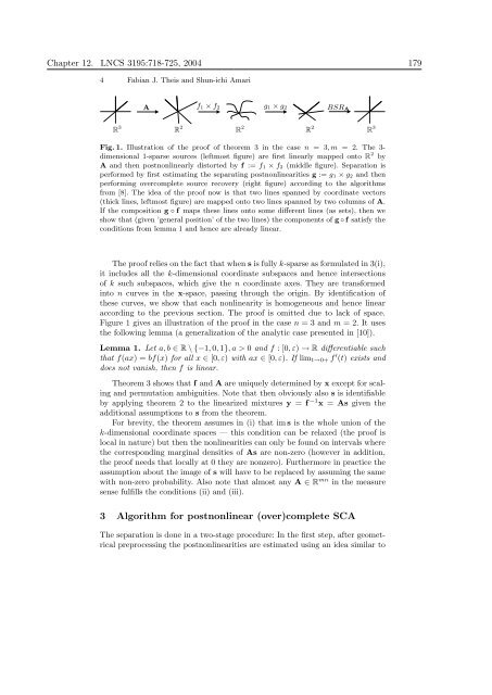
Fig. 1. Illustration of the proof of theorem 3 in the case n = 3, m = 2. The 3dimensional
1-sparse sources (leftmost figure) are first linearly mapped onto R 2 by
A and then postnonlinearly distorted by f := f1 × f2 (middle figure). Separation is
performed by first estimating the separating postnonlinearities g := g1 × g2 and then
performing overcomplete source recovery (right figure) according to the algorithms
from [8]. The idea of the proof now is that two lines spanned by coordinate vectors
(thick lines, leftmost figure) are mapped onto two lines spanned by two columns of A.
If the composition g ◦ f maps these lines onto some different lines (as sets), then we
show that (given ’general position’ of the two lines) the components of g ◦ f satisfy the
conditions from lemma 1 and hence are already linear.
The proof relies on the fact that when s is fully k-sparse as formulated in 3(i),
it includes all the k-dimensional coordinate subspaces and hence intersections
of k such subspaces, which give the n coordinate axes. They are transformed
into n curves in the x-space, passing through the origin. By identification of
these curves, we show that each nonlinearity is homogeneous and hence linear
according to the previous section. The proof is omitted due to lack of space.
Figure 1 gives an illustration of the proof in the case n = 3 and m = 2. It uses
the following lemma (a generalization of the analytic case presented in [10]).
Lemma 1. Let a, b ∈ R \ {−1, 0, 1}, a > 0 and f : [0, ε) → R differentiable such
that f(ax) = bf(x) for all x ∈ [0, ε) with ax ∈ [0, ε). If limt→0+ f ′ (t) exists and
does not vanish, then f is linear.
Theorem 3 shows that f and A are uniquely determined by x except for scaling
and permutation ambiguities. Note that then obviously also s is identifiable
by applying theorem 2 to the linearized mixtures y = f −1 x = As given the
additional assumptions to s from the theorem.
For brevity, the theorem assumes in (i) that im s is the whole union of the
k-dimensional coordinate spaces — this condition can be relaxed (the proof is
local in nature) but then the nonlinearities can only be found on intervals where
the corresponding marginal densities of As are non-zero (however in addition,
the proof needs that locally at 0 they are nonzero). Furthermore in practice the
assumption about the image of s will have to be replaced by assuming the same
with non-zero probability. Also note that almost any A ∈ R mn in the measure
sense fulfills the conditions (ii) and (iii).
3 Algorithm for postnonlinear (over)complete SCA
The separation is done in a two-stage procedure: In the first step, after geometrical
preprocessing the postnonlinearities are estimated using an idea similar to
R 2
R 3