Mathematics in Independent Component Analysis

Chapter 18. Proc. EUSIPCO 2006 249
v1 − v0,...,vn − v0 are linearly independent. Consider the
following embedding
R n → R n+1 : (x1,...,xn) ↦→ (x1,...,xn,1).
We may therefore identify the p dimensional affine subspaces
with the p + 1 linear subspaces in R n+1 by embedding
the generators and taking the linear closure. In fact it
is easy to see that we obtain a 1-to-1 mapping between the
p dimensional affine subspaces of R n and the p + 1 dimensional
linear subspaces in R n−1 , which intersect the orthogonal
complement of (0,...,0,1) only at the origin.
Hence we can reduce the affine case to calculations for
linear subsets only. Note that since only eigenvectors of sums
of projections onto the subsets Vi can become centroids in
the batch version of the k-means algorithm, any centroid is
also in the image of the above embedding and can be identified
uniquely with a affine subspace of the original problem.
4. EXPERIMENTAL RESULTS
We finish by illustrating the algorithm in a few examples.
4.1 Toy example
As a toy example, let us first consider 10 4 samples of
G4,2, namely uniformly randomly chosen from the 6 possible
2-dimensional coordinate planes. In order to avoid
any bias within the algorithm, the non-zero coefficients from
the plane-representing matrices have been chosen uniformly
from O2. The samples have been deteriorated by Gaussian
noise with a signal-to-noise ratio of 10dB. Application of
the Grassmann k-means algorithm with k = 6 yields convergence
after only 6 epochs with the resulting 6 clusters
with centroids [V i ]. The distance measure µ(V) := (|vi1 +
vi2| + |vi1 − vi2|)i should be large only in two coordinates if
[V] is close to the corresponding 2-dimensional coordinate
plane. And indeed, the found centroids have distance measures
µ(V i ) =
⎛ ⎞ ⎛ ⎞ ⎛ ⎞ ⎛ ⎞ ⎛ ⎞ ⎛ ⎞
0.02 1.7 1.7 0.01 2.0 0.01
⎜ 0 ⎟ ⎜0.01⎟
⎜0.01⎟
⎜ 1.5 ⎟ ⎜ 2.0 ⎟ ⎜ 2.0 ⎟
⎝
1.9
⎠, ⎝
0.01
⎠, ⎝
1.7
⎠, ⎝
1.5
⎠, ⎝
0
⎠, ⎝
0.01
⎠.
1.9 1.7 0.02 0 0.01 2.0
Hence, the algorithm correctly chose all 6 coordinate planes
as cluster centroids.
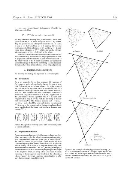
4.2 Polytope identification
As an example application of the Grassmann clustering algorithm,
we want to solve the following approximation problem
from computational geometry: given a set of points, identify
the smallest convex polytope with a fixed number of faces
k, containing the points. In two dimensions, this implies the
task of finding the k edges of a polytope where only samples
in the inside are known. We use QHull algorithm [1] to
construct the convex hull thus identifying the possible edges
of the polytope. Then, we apply affine Grassmann k-means
clustering to these edges in order to identify the k bounding
edges. Figure 4 shows an example. Generalization to arbitrary
dimensions are straight-forward.
(a) Samples (b) QHull
(c) Grassmann clustering
(d) Result
Samples
QHull contour
Grasmann clustering
Mixing matrix
Figure 4: An example of using hyperplane clustering (p =
n − 1) to identify the contour of a samples figure. QHull was
used to find the outer edges then those are clustered into 4
clusters. The broken lines show the boundaries use to generate
the 300 samples.