Mathematics in Independent Component Analysis

242 Chapter 17. IEEE SPL 13(2):96-99, 2006
IEEE SIGNAL PROCESSING LETTERS, VOL. X, NO. XX, XXXX 3
4000
3000
2000
1000
2° 74° 104° 135°
0
0 20 40 60 80 100 120 140 160 180
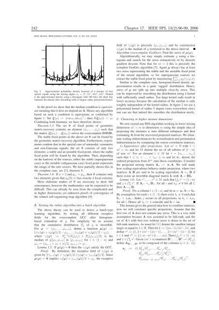
Fig. 2. Approximated probability density function of a mixture of four
speech signals using the mixing angles αi = 2 ◦ ,74 ◦ ,104 ◦ ,135 ◦ . Plotted
is the approximated density using a histogram with 180 bins; the thick line
indicates the density after smoothing with a 5 degree radius polynomial kernel.
In the proof we show that the median-condition is equivariant
meaning that it does no depend on A. Hence any algorithm
based on such a condition is equivariant, as confirmed by
figure 1. Set ξ(ω) := (cosω, sin ω) ⊤ ; then θ(ξ(ω)) = ω.
Combining both lemmata, we have therefore shown:
Theorem 1.3: The set Φ of fixed points of geometric
matrix-recovery contains an element (ˆω1, . . . , ˆωn) such that
the matrix (ξ(ˆω1)...ξ(ˆωn)) solves the overcomplete BMMR.
The stable fixed points in the above set Φ can be found by
the geometric matrix-recovery algorithm. Furthermore, experiments
confirm that in the special case of unimodal, symmetric
and non-Gaussian signals, the set Φ consists of only two
elements: a stable and an unstable fixed point, where the stable
fixed point will be found by the algorithm. Then, depending
on the kurtosis of the sources, either the stable (supergaussian
case) or the instable (subgaussian case) fixed point represents
the image of the unit vectors. We have partially shown this in
the complete case, see [7], theorem 5:
Theorem 1.4: If n = 2 and ps1 = ps2, then Φ contains only
two elements given that py|[0, π) has exactly 4 local extrema.
More elaborate studies of Φ are necessary to show full
convergence, however the mathematics can be expected to be
difficult. This can already be seen from the complicated and
in higher dimensions yet unknown proofs of convergence of
the related self-organizing-map algorithm [9].
B. Turning the online algorithm into a batch algorithm
The above theory can be used to derive a batch-type
learning algorithm, by testing all different receptive
fields for the overcomplete GCC after histogrambased
estimation of y. For simplicity let us assume
that the cumulative distribution Py of y is invertible.
For ϕ = (ϕ1, . . . , ϕn−1), define a function µ(ϕ) :=
((γ1(ϕ) + γ2(ϕ))/2 − ϕ1, . . . , (γn(ϕ) + γ1(ϕ))/2 − ϕn),
where γi(ϕ) := P −1
y ((Py(ϕi) + Py(ϕi+1)/2) is the
median of y|[ϕi, ϕi+1] in [ϕi, ϕi+1] for i ∈ [1 : n] and
ϕn := (ϕn−1 + ϕ1 + π)/2, ϕn+1 := ϕ1.
Lemma 1.5: If µ(ϕ) = 0 then the γi(ϕ) satisfy the GCC.
Proof: By definition, the receptive field of γi(ϕ) is
given by [(γi−1(ϕ) + γi(ϕ))/2, (γi(ϕ) + γi+1(ϕ))/2]. Since
µ(ϕ) = 0 implies γi(ϕ) + γi+1(ϕ))/2 = ϕi, the receptive
field of γi(ϕ) is precisely [ϕi, ϕi+1], and by construction
γi(ϕ) is the median of y restricted to the above interval.
Algorithm (overcomplete FastGeo): Find the zeros of µ(ϕ).
Algorithmically, we may simply estimate y using a histogram
and search for the zeros exhaustively or by discrete
gradient descent. Note that for m = 2 this is precisely the
complete FastGeo algorithm [7]. Again µ always has at least
two zeros representing the stable and the unstable fixed point
of the neural algorithm, so for supergaussian sources we
extract the stable fixed point by maximizing �n i=1 py(γi(ϕi)).
Similar to the complete case, histogram-based density approximation
results in a quite ‘ragged’ distribution. Hence,
zeros of µ are split up into multiple close-by zeros. This
can be improved by smoothing the distribution using a kernel
with sufficiently small radius. Too large kernel radii result in
lower accuracy because the calculation of the median is only
roughly independent of the kernel radius. In figure 2 we use a
polynomial kernel of radius 5 degree (zero everywhere else);
one can see that indeed this smoothes the distribution nicely.
C. Clustering in higher mixture dimensions
We now extend any BSS algorithm working in lower mixing
dimension m ′ < m to dimension m using the simple idea of
projecting the mixtures x onto different subspaces and then
estimating A from the recovered projected matrices. We eliminate
scaling indeterminacies by normalization and permutation
indeterminacies by comparing the source correlation matrices.
1) Equivalence after projections: Let m ′ ∈ N with 1 <
m ′ < m, and let M denote the set of all subsets of [1 : m]
of size m ′ . For an element τ ∈ M let τ = {τ1, . . . , τm ′}
such that 1 ≤ τ1 < . . . < τm ′ ≤ m and let πτ denote the
ordered projection from R m onto those coordinates. Consider
the projected mixing matrix Aτ := πτA. We will study
how scaling-equivalence behaves under projection, where two
matrices A,B are said to be scaling equivalent, A ∼s B if
there exists an invertible diagonal matrix L with A = BL.
Lemma 1.6: Let τ 1 , . . . , τ k ∈ M such that �
i τi = [1 : m]
and j ∈ �
i τi . If A τ i ∼s B τ i for all i and ajl �= 0 for all l,
then A ∼s B.
Proof: Fix a column l ∈ [1 : n], and let a := al, b := bl.
By assumption, for each i ∈ [1 : k] there exist λi �= 0 such that
b τ i = λia τ i. Index j occurs in all projections, so bj = λiaj
for all i. Hence all λi =: λ coincide and b = λa.
This lemma gives the general idea how to combine matrices;
now we will construct specific projections. Assume that the
first row of A does not contain any zeros. This is a very mild
assumption because A was assumed to be full-rank, and the
set of A’s with first row without zeros is dense in the set of
full-rank matrices. As usual let ⌈λ⌉ denote the smallest integer
larger or equal to λ ∈ R. Then let k := ⌈(m−1)/(m ′ −1)⌉, and
define τ i := {1, 2+(m ′ −1)(i−1), . . .,2+(m ′ −1)i−1} for
i < k and τ k := {1, m−m ′ +2, . . ., m}. Then �
i τi = [1 : m]
and 1 ∈ �
i τi . Given (m ′ ×n)-matrices B 1 , . . .,B k := (b k i,j ),
define A B 1 ,...,B k to be composed of the columns (j ∈ [1 : n])
aj := (1, b 1 2,j /b1 1,j , . . . , b1 m ′ ,j /b1 1,j ,
b 2 2,j /b21,j , . . . , bk−1
m ′ ,j /bk−1 1,j ,
b k 3+k(m ′ −1)−m,j /bk1,j , . . . , bkm ′ ,j /bk1,j )⊤ .