Mathematics in Independent Component Analysis

Chapter 11. EURASIP JASP, 2007 167
6 EURASIP Journal on Advances in Signal Processing
x3
3
2.5
2
1.5
1
2
1.5
10.5
00.5
x2 11.5
2 2
(a) Data space
3
4
x1
5
6
θ
3
2.5
2
1.5
1
0.5
0
0 0.5 1 1.5 2 2.5 3
ϕ
(b) Spherical Hough space
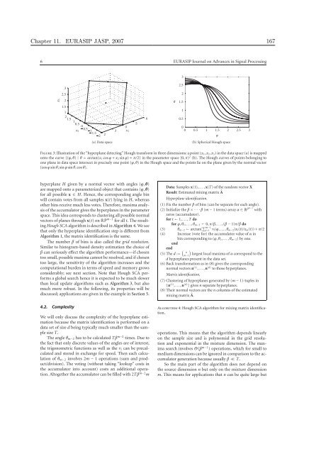
Figure 3: Illustration of the “hyperplane detecting” Hough transform in three dimensions: a point (x1, x2, x3) in the data space (a) is mapped
onto the curve {(ϕ, θ) | θ = arctan(x1 cos ϕ + x2 sin ϕ) + π/2} in the parameter space [0, π) 2 (b). The Hough curves of points belonging to
one plane in data space intersect in precisely one point (ϕ, θ) in the Hough space and the points lie on the plane given by the normal vector
(cos ϕ sin θ, sin ϕ sin θ, cos θ).
hyperplane H given by a normal vector with angles (ϕ, θ)
are mapped onto a parameterized object that contains (ϕ, θ)
for all possible x ∈ H. Hence, the corresponding angle bin
will contain votes from all samples x(t) lying in H, whereas
other bins receive much less votes. Therefore, maxima analysis
of the accumulator gives the hyperplanes in the parameter
space. This idea corresponds to clustering all possible normal
vectors of planes through x(t) on RP m−1 for all t. The resulting
Hough SCA algorithm is described in Algorithm 4. We see
that only the hyperplane identification step is different from
Algorithm 1, the matrix identification is the same.
The number β of bins is also called the grid resolution.
Similar to histogram-based density estimation the choice of
β can seriously effect the algorithm performance—if chosen
too small, possible maxima cannot be resolved, and if chosen
too large, the sensitivity of the algorithm increases and the
computational burden in terms of speed and memory grows
considerably; see next section. Note that Hough SCA performs
a global search hence it is expected to be much slower
than local update algorithms such as Algorithm 3, but also
much more robust. In the following, its properties will be
discussed; applications are given in the example in Section 5.
4.2. Complexity
We will only discuss the complexity of the hyperplane estimation
because the matrix identification is performed on a
data set of size d being typically much smaller than the sample
size T.
The angle θm−2 has to be calculated Tβ m−2 times. Due to
the fact that only discrete values of the angles are of interest,
the trigonometric functions as well as the νi can be precalculated
and stored in exchange for speed. Then each calculation
of θm−2 involves 2m − 1 operations (sum and product/division).
The voting (without taking “lookup” costs in
the accumulator into account) costs an additional operation.
Altogether the accumulator can be filled with 2Tβ m−2 m
Data: Samples x(1), . . . , x(T) of the random vector X
Result: Estimated mixing matrix �A
Hyperplane identification.
(1) Fix the number β of bins (can be separate for each angle).
(2) Initialize the β × · · · β (m − 1 terms) array α ∈ Rβm−1 with
zeros (accumulator).
for t ← 1, . . . , T do
for ϕ, θ1, . . . , θm−3 ← 0, π/β, . . . , (β − 1)π/β do
(3) θm−2 ← arctan( �m−1 i=1 νi(ϕ, . . . , θm−3)xi(t)/xm(t)) + π/2
(4) Increase (vote for) the accumulator value of α in
bin corresponding to (ϕ, θ1, . . . , θm−2) by one.
end
end � �
n
(5) The d := m−1 largest local maxima of α correspond to the
d hyperplanes present in the data set.
(6) Back transformation as in (8) gives the corresponding
normal vectors n (1) , . . . , n (d) to those hyperplanes.
Matrix identification.
(7) Clustering of hyperplanes generated by (m − 1)-tuples in
{n (1) , . . . , n (d) } gives n separate hyperplanes.
(8) Their normal vectors are the n columns of the estimated
mixing matrix �A.
Algorithm 4: Hough SCA algorithm for mixing matrix identification.
operations. This means that the algorithm depends linearly
on the sample size and is polynomial in the grid resolution
and exponential in the mixture dimension. The maxima
search involves O(β m−1 ) operations, which for small to
medium dimensions can be ignored in comparison to the accumulator
generation because usually β ≪ T.
So the main part of the algorithm does not depend on
the source dimension n but only on the mixture dimension
m. This means for applications that n can be quite large but