Mathematics in Independent Component Analysis

Chapter 11. EURASIP JASP, 2007 169
8 EURASIP Journal on Advances in Signal Processing
5
0
5
10
0
5
100 200 300 400 500 600 700 800 900 1000
0
5
0 100 200 300 400 500 600 700 800 900 1000
5
0
5
0
10
5
0
100 200 300 400 500 600 700 800 900 1000
5
0 100 200 300 400 500 600 700 800 900 1000
1
0.5
0
0.5
1
1
0.5
0
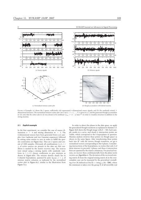
(a) Source signals
0.5
1 1
0.5
(c) Normalized mixture scatter plot
0
0.5
1
5
0
5
10
0
4
2
0
100 200 300 400 500 600 700 800 900 1000
2
4
0
5
100 200 300 400 500 600 700 800 900 1000
0
5
0 100 200 300 400 500 600 700 800 900 1000
50
100
150
200
250
300
350
(b) Mixture signals
50 100 150 200 250 300 350
(d) Hough accumulator with labeled maxima
Figure 4: Example: (a) shows the 2-sparse, sufficiently rich represented, 4-dimensional source signals, and (b) the randomly mixed, 3dimensional
mixtures. The normalized mixture scatter plot {x(t)/|x(t)| | t = 1, . . . , T} is given in (c), and the generated Hough accumulator
in (d); note that the color scale in (d) was chosen to be nonlinear (γnew := (1 − γ/ max) 10 ) in order to visualize structure in addition to the
strong maxima.
5.1. Explicit example
In the first experiment, we consider the case of source dimensions
n = 4 and mixing dimension m = 3. The
4-dimensional sources have been generated from i.i.d. samples
(two Laplacian and two Gaussian sequences) followed
by setting some entries to zero in order to fulfill the sparsity
constraints; see Figure 4(a). They are 2-sparse and consist
of 1000 samples. Obviously all combinations (i, j), i <
j, of active sources are present in the data set; this condition
is needed by the matrix recovery step. The sources
were mixed using a mixing matrix with randomly (uniform
in [−1, 1]) chosen coefficients to give mixtures as
shown in Figure 4(b). The mixture density clearly lies in
6 disjoint hyperplanes, spanned by pairs (ai, aj), i < j, of
mixture matrix columns, as indicated by the normalized
scatter plot in Figure 4(c), similar to the illustration from
Figure 1(c).
In order to detect the planes in the data space, we apply
the generalized Hough transform as explained in Section 3.3.
Figure 4(d) shows the Hough image with β = 360. Each sample
results in a curve, and clearly 6 intersection points are
visible, which correspond to the 6 hyperplanes in question.
Maxima analysis retrieves these points (in Hough space) as
shown in the same figure. After transforming these points
back into R 3 with the inverse Hough transform, we get 6
normalized vectors corresponding to the 6 planes. Considering
intersections of the hyperplanes, we notice that only 4 of
them intersect in precisely 3 planes, and these 4 intersection
lines are spanned by the matrix columns ai. For practical reasons,
we recover these combinatorially from the plane norm
vectors; see Algorithm 4. The deviation of the recovered mixing
matrix �A from the original mixing matrix A in the overcomplete
case can be measured by the generalized crosstalking
error [8] defined as E(A, �A) := minM∈Π �A− �AM�, where
the minimum is taken over the group Π of all invertible real
180
160
140
120
100
80
60
40
20