Mathematics in Independent Component Analysis

166 Chapter 11. EURASIP JASP, 2007
Fabian J. Theis et al. 5
for x ∈ R m with xm �= 0 and
⎧
m−3 �
cos ϕ sin θj, i = 1,
j=1
⎪⎨ m−3 �
νi := sin ϕ sin θj, i = 2,
j=1
�i−2
m−3 �
⎪⎩
cos θj sin θj, i > 2.
j=1 j=i−1
(10)
With cot(θ + π/2) = − tan(θ) we finally get θm−2 = arctan
( �m−1 i=1 νixi/xm) + π/2. Note that continuity is achieved if we
set θm−2 := 0 for xm = 0.
We can then define the generalized “hyperplane detecting”
Hough transform as
x ↦−→
�
η[ fh] : R m −→ P �
[0, π) m−1�
,
(ϕ, θ1, . . . , θm−2)
∈ [0, π) m−1 | θm−2 = arctan
� m−1 �
� xi
νi
xm i=1
+ π
�
.
2
(11)
The parametrization fh is separating, so points lying on the
same hyperplane are mapped to surfaces that intersect in precisely
one point in [0, π) m−1 . This is demonstrated in the case
m = 3 in Figure 3. The hyperplane structures of a data set
X = {x(1), . . . , x(T)} can be analyzed by finding clusters in
η[ fh](X).
Let RP m−1 denote the (m − 1)-dimensional real projective
space, that is, the manifold of all 1-dimensional subspaces
of R m . There is a canonical diffeomorphism between RP m−1
and the Grassmanian manifold of all (m − 1)-dimensional
subspaces of R m , induced by the scalar product. Using this
diffeomorphism, we can reformulate our aim of identifing
hyperplanes as finding elements of RP m−1 . So, the Hough
transform η[ fh] maps x onto a subset of RP m−1 , which is
topologically equivalent to the upper hemisphere in R m with
identifications along the boundary. In fact, in (11) we simply
have constructed a coordinate map of RP m−1 using spherical
coordinates.
4. HOUGH SCA ALGORITHM
The SCA matrix detection algorithm � (Algorithm � 1) consists
n
of two steps. In the first step, d := m−1 hyperplanes given
by their normal vectors n (1) , . . . , n (d) are constructed such
that the mixture data lies in the union of these hyperplanes—
in the case of noise this will hold only approximately. In the
second step, mixture matrix columns ai are identified as generators
of the n lines lying at the intersections of � �
n−1
m−2 hyperplanes.
We replace the first step by the following Hough
SCA algorithm.
x2
a2
ρ
15
10
5
0
5
10
0 1 2 3 4 5 6 7 8 9 10
15
10
5
0
5
10
15
x1
(a) Data space
20
0 0.5 1 1.5 2 2.5 3
20
15
10
5
0
5
10
a1
(b) Linear Hough space
0 0.5 1 1.5 2 2.5 3
θ
(c) Polar Hough space
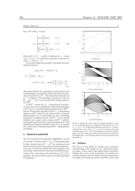
Figure 2: Illustration of the “classical” Hough transform: a point
(x1, x2) in the data space (a) is mapped (b) onto the line {(a1, a2) |
a2 = −a1x1 + x2} in the linear parameter space R 2 or (c) onto a
translated sine curve {(θ, ρ) | ρ = x1 cos θ + x2 sin θ} in the polar
parameter space [0, π) × R + 0 . The Hough curves of points belonging
to one line in data space intersect in precisely one point a in
the Hough space—and the data points lie on the line given by the
parameter a.
4.1. Definition
The idea is to first gather the Hough curves η[ fh](x(t))
corresponding to the samples x(t) in a discretized parameter
space, in this context often called Hough accumulator.
Plotting these curves in the accumulator is sometimes denoted
as voting for each bin, similar to histogram generation.
According to the previous section, all points x from some