Mathematics in Independent Component Analysis

Chapter 12. LNCS 3195:718-725, 2004 181
6 Fabian J. Theis and Shun-ichi Amari
for an unknown constant c �= 0, ±1 and given curves y, z : (−1, 1) → R with
y(0) = z(0) = 0. By theorem 3, g (and also c) are uniquely determined by
y and z except for scaling. Indeed by taking derivatives in equation 3, we get
c = y ′ (0)/z ′ (0), so c can be directly calculated from the known curves y and z.
In the following section, we propose to solve this problem numerically, given
samples y(t1), z(t1), . . . , y(tT ), z(tT ) of the curves. Note that here it is assumed
that the samples of the curves y and z are given at the same time instants
ti ∈ (−1, 1). In practice, this is usually not the case, so values of z at the sample
points of y and vice versa will first have to be estimated, for example by using
spline interpolation.
3.3 MLP-based postnonlinearity approximation
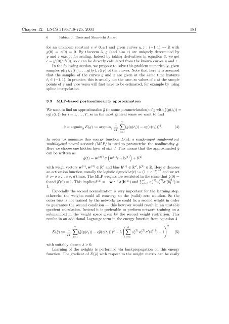
We want to find an approximation ˜g (in some parametrization) of g with ˜g(y(ti)) =
c˜g(z(ti)) for i = 1, . . . , T , so in the most general sense we want to find
˜g = argmin g E(g) := argmin g
1
2T
T�
(g(y(ti)) − cg(z(ti))) 2 . (4)
In order to minimize this energy function E(g), a single-input single-output
multilayered neural network (MLP) is used to parametrize the nonlinearity g.
Here we choose one hidden layer of size d. This means that the approximated ˜g
can be written as
˜g(t) = w (2)⊤ �
¯σ w (1) t + b (1)�
+ b (2)
with weigh vectors w (1) , w (2) ∈ R d and bias b (1) ∈ R d , b (2) ∈ R. Here σ denotes
an activation function, usually the logistic sigmoid σ(t) := (1 + e −t ) −1 and we set
¯σ := σ×. . .×σ, d times. The MLP weights are restricted in the sense that ˜g(0) =
0 and ˜g ′ (0) = 1. This implies b (2) = −w (2)⊤¯σ(b (1) ) and �d i=1 w(1) i w(2) i σ′ (b (1)
1 ) =
1.
Especially the second normalization is very important for the learning step,
otherwise the weights could all converge to the (valid) zero solution. So the
outer bias is not trained by the network; we could fix a second weight in order
to guarantee the second condition — this however would result in an unstable
quotient calculation. Instead it is preferable to perform network training on a
submanifold in the weight space given by the second weight restriction. This
results in an additional Lagrange term in the energy function from equation 4
Ē(˜g) := 1
2T
i=1
T�
(˜g(y(tj)) − c˜g(z(tj))) 2 �
d�
+ λ
j=1
i=1
w (1)
i w(2) i σ′ (b (1)
1
) − 1
with suitably chosen λ > 0.
Learning of the weights is performed via backpropagation on this energy
function. The gradient of Ē(˜g) with respect to the weight matrix can be easily
�2
(5)