Mathematics in Independent Component Analysis

More documents

Recommendations

Info

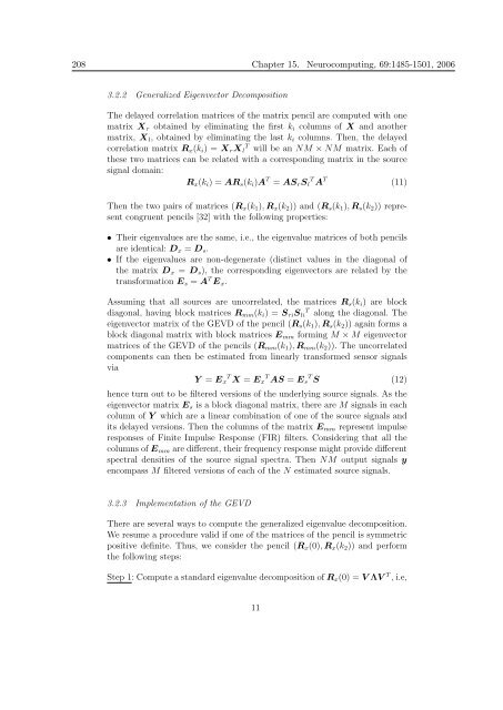
208 Chapter 15. Neurocomputing, 69:1485-1501, 2006 3.2.2 Generalized Eigenvector Decomposition The delayed correlation matrices of the matrix pencil are computed with one matrix Xr obtained by eliminating the first ki columns of X and another matrix, Xl, obtained by eliminating the last ki columns. Then, the delayed correlation matrix Rx(ki) = XrXl T will be an NM × NM matrix. Each of these two matrices can be related with a corresponding matrix in the source signal domain: Rx(ki) = ARs(ki)A T = ASrSl T A T (11) Then the two pairs of matrices (Rx(k1), Rx(k2)) and (Rs(k1), Rs(k2)) represent congruent pencils [32] with the following properties: • Their eigenvalues are the same, i.e., the eigenvalue matrices of both pencils are identical: Dx = Ds. • If the eigenvalues are non-degenerate (distinct values in the diagonal of the matrix Dx = Ds), the corresponding eigenvectors are related by the transformation Es = A T Ex. Assuming that all sources are uncorrelated, the matrices Rs(ki) are block diagonal, having block matrices Rmm(ki) = SriSli T along the diagonal. The eigenvector matrix of the GEVD of the pencil (Rs(k1), Rs(k2)) again forms a block diagonal matrix with block matrices Emm forming M × M eigenvector matrices of the GEVD of the pencils (Rmm(k1), Rmm(k2)). The uncorrelated components can then be estimated from linearly transformed sensor signals via Y = Ex T X = Ex T AS = Es T S (12) hence turn out to be filtered versions of the underlying source signals. As the eigenvector matrix Es is a block diagonal matrix, there are M signals in each column of Y which are a linear combination of one of the source signals and its delayed versions. Then the columns of the matrix Emm represent impulse responses of Finite Impulse Response (FIR) filters. Considering that all the columns of Emm are different, their frequency response might provide different spectral densities of the source signal spectra. Then NM output signals y encompass M filtered versions of each of the N estimated source signals. 3.2.3 Implementation of the GEVD There are several ways to compute the generalized eigenvalue decomposition. We resume a procedure valid if one of the matrices of the pencil is symmetric positive definite. Thus, we consider the pencil (Rx(0), Rx(k2)) and perform the following steps: Step 1: Compute a standard eigenvalue decomposition of Rx(0) = V ΛV T , i.e, 11
Chapter 15. Neurocomputing, 69:1485-1501, 2006 209 compute the eigenvectors vi and eigenvalues λi. As the matrix is symmetric positive definite, the eigenvalues can be arranged in descending order (λ1 > λ2 > · · · > λNM). This procedure corresponds to the usual whitening step in many ICA algorithms. It can be used to estimate the number of sources, but it can also be considered a strategy to reduce noise much like with PCA denoising. Dropping small eigenvalues amounts to a projection from a highdimensional feature space onto a lower dimensional manifold representing the signal+noise subspace. Thereby it is tacitly assumed that small eigenvalues are related with noise components only. Here we consider a variance criterion to choose the most significant eigenvalues, those related with the embedded deterministic signal, according to λ1 + λ2 + ... + λl λ1 + λ2 + ...λNM ≥ T H (13) If we are interested in the eigenvectors corresponding to directions of high variance of the signals, the threshold T H should be chosen such that their maximum energy is preserved. Similar to the whitening phase in many BSS algorithms, the data matrix X can be transformed using 1 − Q = Λ 2 V T (14) to calculate a transformed matrix of delayed correlations C(k2) to be used in the next step. The transformation matrix can be computed using either the l most significant eigenvalues, in which case denoising is achieved, or all eigenvalues and respective eigenvectors. Also note, that Q represents a l×NM matrix if denoising is considered. Step 2: Use the transformed delayed correlation matrix C(k2) = QRx(k2)Q T and its standard eigenvalue decomposition: the eigenvector matrix U and eigenvalue matrix Dx. The eigenvectors of the pencil (Rx(0), Rx(k2)), which are not normalized, form the columns of the eigenvector matrix Ex = QT 1 − U = V Λ 2 U. The ICs of the delayed sensor signals can then be estimated via the transformation given below, yielding l (or NM) signals, one signal per row of Y : Y = Ex T X = U T QX = U T 1 − Λ 2 V T X (15) The first step of this algorithm is therefore equivalent to a PCA in a highdimensional feature space [9,38], where a matrix similar to Q is used to project the data onto the signal manifold. 12
Page 1 and 2:
Statistical machine learning of bio
Page 3:
to Jakob
Page 6 and 7:
vi Preface
Page 8 and 9:
viii CONTENTS 3 Signal Processing 8
Page 11 and 12:
Chapter 1 Statistical machine learn
Page 13 and 14:
1.1. Introduction 5 auditory cortex
Page 15 and 16:
1.2. Uniqueness issues in independe
Page 17 and 18:
1.2. Uniqueness issues in independe
Page 19 and 20:
S U M M A R Y T his �le contains
Page 21 and 22:
1.3. Dependent component analysis 1
Page 23 and 24:
Table 1.1: BSS algorithms based on
Page 25 and 26:
Page 27 and 28:
Page 29 and 30:
Page 31 and 32:
Page 33 and 34:
1.4. Sparseness 25 1.4 Sparseness O
Page 35 and 36:
1.4. Sparseness 27 Theorem 1.4.3 (S
Page 37 and 38:
1.4. Sparseness 29 R 3 R 3 A BSRA R
Page 39 and 40:
1.4. Sparseness 31 Sparse projectio
Page 41 and 42:
1.5. Machine learning for data prep
Page 43 and 44:
Page 45 and 46:
Page 47 and 48:
Page 49 and 50:
Page 51 and 52:
1.6. Applications to biomedical dat
Page 53 and 54:
Page 55 and 56:
Page 57 and 58:
Page 59 and 60:
1.7. Outlook 51 noise data signal i
Page 61:
Part II Papers 53
Page 64 and 65:
56 Chapter 2. Neural Computation 16
Page 66 and 67:
Page 68 and 69:
Page 70 and 71:
Page 72 and 73:
Page 74 and 75:
Page 76 and 77:
Page 78 and 79:
Page 80 and 81:
Page 82 and 83:
Page 84 and 85:
Page 86 and 87:
Page 88 and 89:
Page 90 and 91:
82 Chapter 3. Signal Processing 84(
Page 92 and 93:
Page 94 and 95:
Page 96 and 97:
Page 98 and 99:
90 Chapter 4. Neurocomputing 64:223
Page 100 and 101:
Page 102 and 103:
Page 104 and 105:
Page 106 and 107:
Page 108 and 109:
Page 110 and 111:
Page 112 and 113:
104 Chapter 5. IEICE TF E87-A(9):23
Page 114 and 115:
Page 116 and 117:
Page 118 and 119:
Page 120 and 121:
Page 122 and 123:
114 Chapter 6. LNCS 3195:726-733, 2
Page 124 and 125:
116 Chapter 6. LNCS 3195:726-733, 2
Page 126 and 127:
118 Chapter 6. LNCS 3195:726-733, 2
Page 128 and 129:
120 Chapter 6. LNCS 3195:726-733, 2
Page 130 and 131:
122 Chapter 6. LNCS 3195:726-733, 2
Page 132 and 133:
124 Chapter 7. Proc. ISCAS 2005, pa
Page 134 and 135:
Page 136 and 137:
Page 138 and 139:
130 Chapter 8. Proc. NIPS 2006 Towa
Page 140 and 141:
132 Chapter 8. Proc. NIPS 2006 1.3
Page 142 and 143:
134 Chapter 8. Proc. NIPS 2006 stru
Page 144 and 145:
136 Chapter 8. Proc. NIPS 2006 5.5
Page 146 and 147:
138 Chapter 8. Proc. NIPS 2006
Page 148 and 149:
140 Chapter 9. Neurocomputing (in p
Page 150 and 151:
Page 152 and 153:
Page 154 and 155:
Page 156 and 157:
Page 158 and 159:
Page 160 and 161:
Page 162 and 163:
Page 164 and 165:
156 Chapter 10. IEEE TNN 16(4):992-
Page 166 and 167: 158 Chapter 10. IEEE TNN 16(4):992-
Page 168 and 169: 160 Chapter 10. IEEE TNN 16(4):992-
Page 170 and 171: 162 Chapter 11. EURASIP JASP, 2007
Page 184 and 185: 176 Chapter 12. LNCS 3195:718-725,
Page 194 and 195: 186 Chapter 13. Proc. EUSIPCO 2005
Page 200 and 201: 192 Chapter 14. Proc. ICASSP 2006 S
Page 202 and 203: 194 Chapter 14. Proc. ICASSP 2006 A
Page 204 and 205: 196 Chapter 14. Proc. ICASSP 2006
Page 206 and 207: 198 Chapter 15. Neurocomputing, 69:
Page 238 and 239: 230 Chapter 16. Proc. ICA 2006, pag
Page 248 and 249: 240 Chapter 17. IEEE SPL 13(2):96-9
Page 266 and 267:
258 Chapter 19. LNCS 3195:977-984,
Page 268 and 269:
260 Chapter 19. LNCS 3195:977-984,
Page 270 and 271:
262 Chapter 20. Signal Processing 8
Page 272 and 273:
Page 274 and 275:
Page 276 and 277:
Page 278 and 279:
Page 280 and 281:
Page 282 and 283:
Page 284 and 285:
Page 286 and 287:
Page 288 and 289:
Page 290 and 291:
Page 292 and 293:
Page 294 and 295:
Page 296 and 297:
Page 298 and 299:
Page 300 and 301:
292 Chapter 21. Proc. BIOMED 2005,
Page 302 and 303:
Page 304 and 305:
Page 306 and 307:
298 BIBLIOGRAPHY Barber, C., Dobkin
Page 308 and 309:
300 BIBLIOGRAPHY Georgiev, P. (2001
Page 310 and 311:
302 BIBLIOGRAPHY Keck, I., Theis, F
Page 312 and 313:
304 BIBLIOGRAPHY Schießl, I., Sch
Page 314 and 315:
306 BIBLIOGRAPHY Theis, F. and Inou
show all

Mathematics in Independent Component Analysis

You also want an ePaper? Increase the reach of your titles

Delete template?

Save as template?