Mathematics in Independent Component Analysis

1.4. Sparseness 31
Sparse projection
Algorithmically, we followed Hoyer’s approach and solved the
sparse NMF problem by alternatively updating A and S using
gradient descent on the residual error �X − AS� 2 . After each
update, the columns of A and the rows of S are projected onto
M := {s|�s�1 = σ} ∩ {s|�s�2 = 1} ∩ {s ≥ 0} (1.14)
in order to satisfy the sparseness conditions of (1.13). For this,
points x ∈ R n have to be projected onto adjacent points in M,
which was defined as �x − p�2 ≤ �x − q�2 for all q ∈ M and
denoted as p ⊳ x.
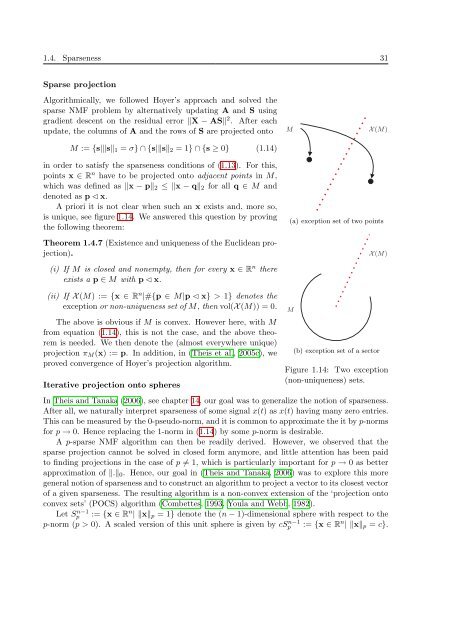
A priori it is not clear when such an x exists and, more so,
is unique, see figure 1.14. We answered this question by proving
the following theorem:
Theorem 1.4.7 (Existence and uniqueness of the Euclidean projection).
M X (M)
(i) If M is closed and nonempty, then for every x ∈ R n there
exists a p ∈ M with p ⊳ x.
(ii) If X (M) := {x ∈ R n |#{p ∈ M|p ⊳ x} > 1} denotes the
exception or non-uniqueness set of M, then vol(X (M)) = 0.
M X (M)
(a) exception set of two points
(a) exception set of two points
M
(b) excepti
Figure 1: Two examples of exception s
In other words, the exception set contains the set of
can’t uniquely project. Our goal is to show that this set
very small. Figure 1 shows the exception set of two diffe
Note that if x ∈ M then x ⊳ x, and x is the only poi
So M ∩ X (M) = ∅. Obviously the exception set of an a
is empty. Indeed, we can prove more generally:
Lemma 2.4. Let M ⊂ Rn X (M)
M
be convex. Then X (M) = ∅.
For the proof we need the following simple lemma, wh
2-norm as it uses the scalar product.
Lemma 2.5. Let a, b ∈ Rn such that �a + b�2 = �a�2 +
are collinear.
Proof. By taking squares we get �a + b�2 = �a�2 + 2�a�
�a� 2 + 2〈a, b〉 + �b� 2 = �a� 2 + 2�a��b� +
if 〈., .〉 denotes the (symmetric) scalar product. Hence 〈
and b are collinear according to the Schwarz inequality.
Proof of lemma 2.4. Assume X (M) �= ∅. Then let x ∈
M such that pi ⊳ x. By assumption q := 1
2 (p1 + p2) ∈ M
�x − p1� ≤ �x − q� ≤ 1
2 �x − p1� + 1
�x − p2�
2
because both pi are adjacent to x. Therefore �x−q� = � 1
(a) exception set of two points
(b) exception set of a sector
Figure 1: Two examples of exception sets.
In other words, the exception set contains the set of points from which we
can’t uniquely project. Our goal is to show that this set vanishes or is at least
very small. Figure 1 shows the exception set of two different sets.
Note that if x ∈ M then x ⊳ x, and x is the only point with that property.
So M ∩ X (M) = ∅. Obviously the exception set of an affine linear hyperspace
is empty. Indeed, we can prove more generally:
Lemma 2.4. Let M ⊂ R
2
and application of lemma 2.5 shows that x − p1 = α(x
3
n be convex. Then X (M) = ∅.
For the proof we need the following simple lemma, which only works for the
2-norm as it uses the scalar product.
Lemma 2.5. Let a, b ∈ Rn such that �a + b�2 = �a�2 + �b�2. Then a and b
are collinear.
Proof. By taking squares we get �a + b�2 = �a�2 + 2�a��b� + �b�2 , so
�a� 2 + 2〈a, b〉 + �b� 2 = �a� 2 + 2�a��b� + �b� 2
The above is obvious if M is convex. However here, with M
from equation (1.14), this is not the case, and the above theorem
is needed. We then denote the (almost everywhere unique)
projection πM(x) := p. In addition, in (Theis et al., 2005c), we (b) exception set of a sector
proved convergence of Hoyer’s projection algorithm.
Figure 1.14: Two exception
(non-uniqueness) sets.
Iterative projection onto spheres
In Theis and Tanaka (2006), see chapter 14, our goal was to generalize the notion of sparseness.
After all, we naturally interpret sparseness of some signal x(t) as x(t) having many zero entries.
This can be measured by the 0-pseudo-norm, and it is common to approximate the it by p-norms
for p → 0. Hence replacing the 1-norm in (1.14) by some p-norm is desirable.
A p-sparse NMF algorithm can then be readily derived. However, we observed that the
sparse projection cannot be solved in closed form anymore, and little attention has been paid
to finding projections in the case of p �= 1, which is particularly important for p → 0 as better
approximation of �.�0. Hence, our goal in (Theis and Tanaka, 2006) was to explore this more
general notion of sparseness and to construct an algorithm to project a vector to its closest vector
of a given sparseness. The resulting algorithm is a non-convex extension of the ‘projection onto
convex sets’ (POCS) algorithm (Combettes, 1993, Youla and Webb, 1982).
Let S
if 〈., .〉 denotes the (symmetric) scalar product. Hence 〈a, b〉 = �a��b� and a
and b are collinear according to the Schwarz inequality.
n−1
p := {x ∈ Rn | �x�p = 1} denote the (n − 1)-dimensional sphere with respect to the
p-norm (p > 0). A scaled version of this unit sphere is given by cSn−1 p := {x ∈ Rn | �x�p = c}.
Proof of lemma 2.4. Assume X (M) �= ∅. Then let x ∈ X (M) and p1 �= p2 ∈
M such that pi ⊳ x. By assumption q := 1
2 (p1 + p2) ∈ M. But
�x − p1� ≤ �x − q� ≤ 1
2 �x − p1� + 1
2 �x − p2� = �x − p1�
(x−p1)�+� 1
2 (x−p2)�
because both pi are adjacent to x. Therefore �x−q� = � 1
2
and application of lemma 2.5 shows that x − p1 = α(x − p2). Taking norms
3