Mathematics in Independent Component Analysis

1.4. Sparseness 29
R 3
R 3
A
BSRA
R 2
R 2
f1 × f2
g1 × g2
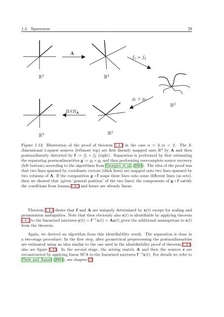
Figure 3: Illustration of the proof of theorem ?? in the case n = 3, m = 2. The 3dimensional
1-sparse sources (leftmost figure) are first linearly mapped onto R2 Figure 1.13: Illustration of the proof of theorem 1.4.4 in the case n = 3, m = 2. The 3dimensional
1-sparse sources (leftmost top) are first linearly mapped onto R by
A and then postnonlinearly distorted by f := f1 × f2 (middle figure). Separation
is performed by first estimating the separating postnonlinearities g := g1 × g2 and
then performing overcomplete source recovery (right figure) according to algorithm
??. The idea of the proof now is that two lines spanned by coordinate vectors (fat
lines, leftmost figure) are mapped onto two lines spanned by two columns of A.
If the composition g ◦ f maps these lines onto some different lines (as sets), then
we show that (given ’general position’ of the two lines) the components of g ◦ f
are homogeneous functions and hence already linear according to lemma ??.
2 by A and then
postnonlinearly distorted by f := f1 × f2 (right). Separation is performed by first estimating
the separating postnonlinearities g := g1 ×g2 and then performing overcomplete source recovery
(left bottom) according to the algorithms from Georgiev et al. (2004). The idea of the proof was
that two lines spanned by coordinate vectors (thick lines) are mapped onto two lines spanned by
two columns of A. If the composition g ◦ f maps these lines onto some different lines (as sets),
then we showed that (given ‘general position’ of the two lines) the components of g ◦ f satisfy
the conditions from lemma 1.4.5 and hence are already linear.
Theorem 1.4.4 shows that f and A are uniquely determined by x(t) except for scaling and
permutation ambiguities. Note that then obviously also s(t) is identifiable by applying theorem
(i) s is fully k-sparse in the sense that im s equals the union of all k-dimensional
1.4.2 to the linearized mixtures y(t) = f
coordinate subspaces (in which it is contained by the sparsity assumption),
−1x(t) = As(t) given the additional assumptions to s(t)
from the theorem.
(ii) A is mixing and not absolutely degenerate,
(iii) every m × m-submatrix of A is invertible.
If x = ˆf( ˆs) is another representation of x as in equation ?? with ˆs satisfying the
same conditions as s, then there exists an invertible scaling L with f = ˆ Again, we derived an algorithm from this identifiability result. The separation is done in
a two-stage procedure: In the first step, after geometrical preprocessing the postnonlinearities
are estimated using an idea similar to the one used in the identifiability proof of theorem 1.4.4,
also see figure 1.13. In the second stage, the mixing matrix A and then the sources s are
reconstructed by applying linear SCA to the linearized mixtures f
f ◦ L, and
−1x(t). For details we refer to
Theis and Amari (2004), see chapter 12.
invertible scaling and permutation matrices L ′ , P ′ with A = L ÂL′ P ′ .
The proof is given in the appendix. It relies on the fact that when s is fully
k-sparse as formulated in theorem ??(??), it includes all the k-dimensional coordinate
subspaces and hence intersections of k such subspaces, which give the
n coordinate axes. They are transformed into n curves in the x-space, passing
through the origin. By identification of these curves, we show that each nonlinearity
is homogeneous and hence linear according to the previous section. Figure
?? gives an illustration of the proof of theorem ?? in the case n = 3 and m = 2.
R 2