Mathematics in Independent Component Analysis

Chapter 7. Proc. ISCAS 2005, pages 5878-5881 125
invariant under these transformations. In [7] we show that
these are the only indeterminacies, given some additional weak
restrictions to the model, namely that A has to be k-admissible
and that s is not allowed to contain a Gaussian k-component.
As usual by preprocessing of the observations x by whitening
we may also assume that Cov(x) = I. Then I =
Cov(x) =A Cov(s)A ⊤ = AA ⊤ so A is orthogonal.
B. MICA using Hessian diagonalization (MHICA)
We assume that s admits a C2−density ps. Using orthogonality
of A we get ps(s0) =px(As0) for s0 ∈ Rnk .Let
Hf (x0) denote the Hessian of f evaluated at x0. It transforms
like a 2-tensor so locally at s0 with ps(s0) > 0 we get
Hln ps (s0)
⊤
=Hln px◦A(s0) =AHln px (As0)A
The key idea now lies in the fact that s is assumed to be kindependent,
so ps factorizes into n groups depending only
on k separate variables each. So ln ps is a sum of functions
depending on k separate variables hence Hln ps (s0) is blockdiagonal
i.e. a k-scaling.
The algorithm, multidimensional Hessian ICA (MHICA),
now simply uses the block-diagonality structure from equation
1 and performs JBD of estimates of a set of Hessians
Hln ps (si) evaluated at different points si ∈ Rnk . Given slight
restrictions on the eigenvalues, the resulting block diagonalizer
then equals A⊤ except for k-scaling and permutation. The
Hessians are estimated using kernel-density approximation
with a sufficiently smooth kernel, but other methods such
as approximation using finite differences are possible, too.
Density approximation is problematic, but in this setting due to
the fact that we can use many Hessians we only need rough
estimates. For more details on the kernel approximation we
refer to the one-dimensional Hessian ICA algorithm from [8].
MHICA generalizes one-dimensional ideas proposed in [8],
[9]. More generally, we could have also used characteristic
functions instead of densities, which leads to a related algorithm,
see [10] for the single-dimensional ICA case.
IV. MULTIDIMENSIONAL TIME DECORRELATION
Instead of assuming k-independence of the sources in
the MBSS problem, in this section we assume that s is a
multivariate centered discrete WSS random process such that
its symmetrized autocovariances
¯Rs(τ) := 1 � � ⊤
E s(t + τ)s(t)
2
� + E � s(t)s(t + τ) ⊤��
(2)
are k-scalings for all τ. This models the fact that the sources
are supposed to be block-decorrelated in the time-domain for
all time-shifts τ.
A. Indeterminacies
Again A can only be found up to k-scaling and kpermutation
because condition 2 is invariant under this transformation.
One sufficient condition for identifiability is to have
pairwise different eigenvalues of at least one Rs(τ), however
generalizations are possible, see [4] for the case k =1.Using
whitening, we can again assume orthogonal A.
(1)
3500
3000
2500
2000
1500
1000
500
0
0.5 1 1.5 2 2.5 3 3.5 4
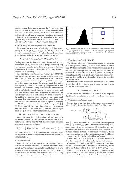
Fig. 1. Histogram and box plot of the multidimensional performance index
E (k) (C) evaluated for k =2and n =2. The statistics were calculated
over 10 5 independent experiments using 4 × 4 matrices C with coefficients
uniformly drawn out of [−1, 1].
B. Multidimensional SOBI (MSOBI)
Theideaofwhatwecallmultidimensional second-order
blind identification (MSOBI) is now a direct extension of the
usual SOBI algorithm [4]. Symmetrized autocovariances of x
can easily be estimated from the data, and they transform as
follows: ¯ Rs(τ) =A⊤ ¯ Rx(τ)A. But ¯ Rs(τ) is a k-scaling by
assumption, so JBD of a set of such symmetrized autocovariance
matrices yields A as diagonalizer (except for k-scaling
and permutation).
Other researchers have worked on this problem in the setting
of convolutive BSS — due to lack of space we want to refer
to [11] and references therein.
V. EXPERIMENTAL RESULTS
In this section we demonstrate the validity of the proposed
algorithms by applying them to both toy and real world data.
A. Multidimensional Amari-index
In order to analyze algorithm performance, we consider the
index E (k) (C) defined for fixed n, k and C ∈ Gl(nk) as
E (k) n�
�
n�
�C
(C) =
r=1 s=1
(k)
rs �
maxi �C (k)
�
− 1
ri �
n�
�
n�
�C
+
s=1 r=1
(k)
rs �
maxi �C (k)
�
− 1 .
is �
Here �.� can be any matrix norm — we choose the operator
norm �A� := max |x|=1 |Ax|. Thismultidimensional performance
index of an nk × nk-matrix C generalizes the onedimensional
performance index introduced by Amari et al. [12]
to block-diagonal matrices. It measures how much C differs
from a permutation and scaling matrix in the sense of k-blocks,
so it can be used to analyze algorithm performance:
Lemma 5.1: Let C ∈ Gl(nk). E (k) (C) =0if and only if
C is the product of a k-scaling and a k-permutation matrix.
Corollary 5.2: Consider the MBSS problem x = As from
section III respectively IV. An estimate  of the mixing matrix
solves the MBSS problem if and only if E (k) ( Â−1 A)=0.
In order to be able to determine the scale of this index, figure
1 gives statistics of E (k) over randomly chosen matrices in the
case k = n =2. The mean is 3.05 and the median 3.10.
4
3.5
3
2.5
2
1.5
1
1