

Mathematics in Independent Component Analysis
Mathematics in Independent Component Analysis
Mathematics in Independent Component Analysis

You also want an ePaper? Increase the reach of your titles
YUMPU automatically turns print PDFs into web optimized ePapers that Google loves.
Chapter 5. IEICE TF E87-A(9):2355-2363, 2004 107<br />
4<br />
where y ′ := Wx and y := Vx.<br />
In applications, V is usually chosen to be the projection<br />
along the first pr<strong>in</strong>cipal components <strong>in</strong> order to<br />
reduce noise [14]. In this case it is easy to see that<br />
<strong>in</strong>deed VA is <strong>in</strong>vertible as needed <strong>in</strong> the theorem.<br />
3. Quadratic ICA<br />
The model of quadratic ICA is <strong>in</strong>troduced and separability<br />
and algorithms are studied <strong>in</strong> this context.<br />
3.1 Model<br />
Let x be an m-dimensional random vector. Consider<br />
the follow<strong>in</strong>g quadratic or bil<strong>in</strong>ear unmix<strong>in</strong>g model<br />
y := g(x, x) (6)<br />
for a fixed bil<strong>in</strong>ear mapp<strong>in</strong>g g : R m × R m → R n .<br />
The components of the bil<strong>in</strong>ear mapp<strong>in</strong>g are quadratic<br />
forms, which can be parameterized by symmetric matrices.<br />
So the above is equivalent to<br />
yi := x ⊤ G (i) x (7)<br />
for symmetric matrices G (i) and i = 1, . . . , n. If G (i)<br />
kl<br />
are the coefficients of G (i) , this means<br />
yi =<br />
m�<br />
m�<br />
k=1 l=1<br />
G (i)<br />
kl xkxl<br />
for i = 1, . . . , n.<br />
A special case of this model can be constructed as<br />
follows: Decompose the symmetric coefficient matrices<br />
<strong>in</strong>to<br />
G (i) = E (i)⊤ Λ (i) E (i) ,<br />
where E (i) is orthogonal and Λ (i) diagonal. In order<br />
to explicitly <strong>in</strong>vert the above model (after restriction<br />
to a subset for <strong>in</strong>vertibility) we now assume that these<br />
coord<strong>in</strong>ate changes E (i) are all the same i.e.<br />
for i = 1, . . . , n. Then<br />
E = E (i)<br />
yi = (Ex) ⊤ Λ (i) (Ex) =<br />
m�<br />
k=1<br />
Λ (i)<br />
kk (Ex)2 k<br />
(8)<br />
where Λ (i)<br />
kk are the coefficients on the diagonal of Λ(i) .<br />
Sett<strong>in</strong>g<br />
⎛<br />
⎜<br />
Λ := ⎝<br />
11 . . . Λ (1) ⎞<br />
nn<br />
. .<br />
. ..<br />
. ⎟<br />
. ⎠<br />
Λ (1)<br />
Λ (n)<br />
11 . . . Λ (n)<br />
nn<br />
yields a two-layered unmix<strong>in</strong>g model<br />
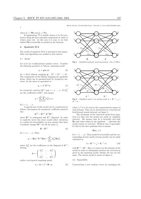
y = Λ ◦ (.) 2 ◦ E ◦ x, (9)<br />
IEICE TRANS. FUNDAMENTALS, VOL.E87–A, NO.9 SEPTEMBER 2004<br />
x1<br />
x2<br />
xm<br />
.<br />
E1m<br />
E2m<br />
Enm<br />
(.) 2<br />
(.) 2<br />
.<br />
(.) 2<br />
Λ1n<br />
Λ2n<br />
E Λ<br />
Λnn<br />
Fig. 1 Simplified quadratic unmix<strong>in</strong>g model y = Λ◦(.) 2 ◦E◦x.<br />
s1<br />
s2<br />
sn<br />
� Λ −1 �<br />
.<br />
1n<br />
�<br />
−1 Λ �<br />
2n<br />
� Λ −1 �<br />
nn<br />
√<br />
√<br />
� E −1 �<br />
.<br />
√<br />
1n<br />
� E −1 �<br />
2n<br />
� E −1 �<br />
Λ −1 E −1<br />
Fig. 2 Simplified square root mix<strong>in</strong>g model x = E −1 ◦ √ ◦<br />
Λ −1 ◦ s.<br />
where (.) 2 is to be read as the componentwise square of<br />
each element. This can be <strong>in</strong>terpreted as a two-layered<br />
feed-forward neural network, see figure 1.<br />
The advantage of the restricted model from equation<br />
8 is that now the model can easily be explicitly<br />
<strong>in</strong>verted. We assume that Λ is <strong>in</strong>vertible and that<br />
Ex only takes values <strong>in</strong> one quadrant — otherwise the<br />
model cannot be <strong>in</strong>verted. Without loss of generality<br />
let this be the first quadrant that is assume<br />
(Ex)i ≥ 0<br />
for i = 1 . . . , m. Then model 9 is <strong>in</strong>vertible and the correspond<strong>in</strong>g<br />
<strong>in</strong>verse model (mix<strong>in</strong>g model) can be easily<br />
expressed as<br />
mn<br />
.<br />
.<br />
y1<br />
y2<br />
yn<br />
x1<br />
x2<br />
xm<br />
x = E −1 ◦ √ ◦ Λ −1 ◦ s (10)<br />
with E −1 = E ⊤ . Here we write s as the doma<strong>in</strong> of the<br />
model <strong>in</strong> order to dist<strong>in</strong>guish between the recoveries y<br />
given by the unmix<strong>in</strong>g model. Ideally, the two are the<br />
same. The <strong>in</strong>verse model is shown <strong>in</strong> figure 2.<br />
3.2 Separability<br />
Construct<strong>in</strong>g a new random vector by arrang<strong>in</strong>g the


