

Mathematics in Independent Component Analysis
Mathematics in Independent Component Analysis
Mathematics in Independent Component Analysis

Create successful ePaper yourself
Turn your PDF publications into a flip-book with our unique Google optimized e-Paper software.
164 Chapter 11. EURASIP JASP, 2007<br />
Fabian J. Theis et al. 3<br />
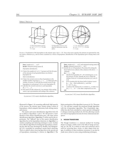
a1<br />
a3<br />
a2<br />
(a) Three hyperplanes span{ai,<br />
aj} for 1 ≤ i < j ≤ 3 <strong>in</strong> the<br />
3 × 3 case<br />
a1<br />
a3<br />
a2<br />
(b) Hyperplanes from (a) visualized<br />
by <strong>in</strong>tersection with the<br />
sphere<br />
a1<br />
a3<br />
a4<br />
a2<br />
(c) Six hyperplanes span{ai,<br />
aj} for 1 ≤ i < j ≤ 4 <strong>in</strong> the<br />
3 × 4 case<br />
Figure 1: Visualization of the hyperplanes <strong>in</strong> the mixture space {x(t)} ⊂ R 3 . Due to the source sparsity, the mixtures are generated by only<br />
two matrix columns ai, aj, and are hence conta<strong>in</strong>ed <strong>in</strong> a union of hyperplanes. Identification of the hyperplanes gives mix<strong>in</strong>g matrix and<br />
sources.<br />
Data: samples x(1), . . . , x(T)<br />
Result: estimated mix<strong>in</strong>g matrix �A<br />
Hyperplane identification.<br />
(1) Cluster the samples x(t) <strong>in</strong> � �<br />
n<br />
m−1 groups such that the span<br />
of the elements of each group produces one dist<strong>in</strong>ct<br />
hyperplane Hi.<br />
Matrix identification.<br />
(2) Cluster the normal vectors to these hyperplanes <strong>in</strong> the<br />
smallest number of groups Gj, j = 1, . . . , n (which gives the<br />
number of sources n) such that the normal vectors to the<br />
hyperplanes <strong>in</strong> each group Gj lie <strong>in</strong> a new hyperplane �Hj.<br />
(3) Calculate the normal vectors �aj to each hyperplane<br />
�Hj, j = 1, . . . , n.<br />
(4) The matrix �A with columns �aj is an estimate of the mix<strong>in</strong>g<br />
matrix (up to permutation and scal<strong>in</strong>g of the columns).<br />
Algorithm 1: SCA matrix identification algorithm.<br />
illustrated <strong>in</strong> Figure 1: by assum<strong>in</strong>g sufficiently high sparsity<br />
of the sources, the mixture space clusters along a union of<br />
hyperplanes, which uniquely determ<strong>in</strong>e both mix<strong>in</strong>g matrix<br />
and sources.<br />
The matrix and source identification algorithm from [9]<br />
are recalled <strong>in</strong> Algorithms 1 and 2. We will present a modification<br />
of the matrix identification part—the same source<br />
identification algorithm (Algorithm 2) will be used <strong>in</strong> the experiments.<br />
The “difficult” part of the matrix identification<br />
algorithm lies <strong>in</strong> the hyperplane detection; <strong>in</strong> Algorithm 1, a<br />
random sampl<strong>in</strong>g and cluster<strong>in</strong>g technique is used. Another<br />
more efficient algorithm for f<strong>in</strong>d<strong>in</strong>g the hyperplanes conta<strong>in</strong><strong>in</strong>g<br />
the data has been developed by Bradley and Mangasarian<br />
[21], essentially by extend<strong>in</strong>g k-means batch cluster<strong>in</strong>g.<br />
Their so-called k-plane cluster<strong>in</strong>g algorithm <strong>in</strong> the special case<br />
of hyperplanes conta<strong>in</strong><strong>in</strong>g 0 is shown <strong>in</strong> Algorithm 3. The<br />
Data: samples x(1), . . . , x(T) and estimated mix<strong>in</strong>g matrix �A<br />
Result: estimated sources �s(1), . . . ,�s(T)<br />
(1) Identify the set of hyperplanes H produced by tak<strong>in</strong>g the<br />
l<strong>in</strong>ear hull of every subsets of the columns of �A with m − 1<br />
elements<br />
for t ← 1, . . . , T do<br />
(2) Identify the hyperplane H ∈ H conta<strong>in</strong><strong>in</strong>g x(t), or, <strong>in</strong><br />
the presence of noise, identify the one to which the<br />
distance from x(t) is m<strong>in</strong>imal and project x(t) onto H<br />
to �x.<br />
(3) If H is produced by the l<strong>in</strong>ear hull of column vectors<br />
�ai1, . . . , �aim−1, f<strong>in</strong>d coefficients λi(j) such that<br />
�x = � m−1<br />
j=1 λi(j)�ai(j).<br />
(4) Construct the solution �s(t): it conta<strong>in</strong>s λi(j) at <strong>in</strong>dex i(j)<br />
for j = 1, . . . , m − 1, the other components are zero.<br />
end<br />
Algorithm 2: SCA source identification algorithm.<br />
f<strong>in</strong>ite term<strong>in</strong>ation of the algorithm is proven <strong>in</strong> [21, Theorem<br />
3.7]. We will later compare the proposed Hough algorithm<br />
with the k-hyperplane algorithm. The k-hyperplane algorithm<br />
has also been extended to a more general, orthogonal<br />
k-subspace cluster<strong>in</strong>g method [22, 23] thus allow<strong>in</strong>g a search<br />
not only for hyperplanes but also for lower-dimensional subspaces.<br />
3. HOUGH TRANSFORM<br />
The Hough transform is a classical method for locat<strong>in</strong>g<br />
shapes <strong>in</strong> images, widely used <strong>in</strong> the field of image process<strong>in</strong>g;<br />
see [10, 24]. It is robust to noise and occlusions and is<br />
used for extract<strong>in</strong>g l<strong>in</strong>es, circles, or other shapes from images.<br />
In addition to these nonl<strong>in</strong>ear extensions, it can also be<br />
made more robust to noise us<strong>in</strong>g antialias<strong>in</strong>g techniques.


