Mathematics in Independent Component Analysis

294 Chapter 21. Proc. BIOMED 2005, pages 209-212
1.5
1
0.5
0
−0.5
−1
−1.5
−2
4
2
0
−2
−4
−3
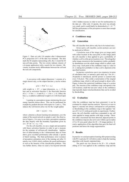
Figure 3. Data set with 120 samples after 3-dimensional
PCA projection (91% of the data was retained). The dots
mark the 60 samples representing cells, the x’s mark the 60
non-cell data points. The two circles indicate clusters of
a k-means application with a search for two clusters. Obviously,
k-means nicely differentiates between the cell and
the non-cell components.
A perceptron with output dimension 1 consists of a
single neuron only, so the output function y can be written
as
y(x) = θ(w ⊤ x + w0)
with weight w ∈ R n , n input dimension, w0 ∈ R the
bias and as activation function θ, the Heaviside function
(θ(x) = 0 for x < 0 and θ(x) = 1 for x ≥ 0). Often, the
bias w0 is added as additional weight to w with fixed input
1.
Learning in a perceptron means minimizing the error
energy function shown above. This can be performed for
example by gradient descent with respect to w and w0. This
induces the well known delta-rule for the weight update
−2
−1
∆w = η(y(x) − t)x,
where η denotes a chosen learning rate parameter, y(x) the
output of the neural network at sample x and t the observation
of input x. It is easy to see that a perceptron separates
the data linearly with the boundary hyperplane given by
{x ∈ R n |w ⊤ x + w0 = 0}.
For the cell classifier, we use a single-unit perceptron
with linear activation function in order to get a measure
for the certainty of cell/non-cell classification. Application
of delta-learning to the 5-dimensional data set from
above gives excellent performance after already 4 epochs
of batch learning. The final performance error (variance
of perceptron estimation error of the training set) after 55
epochs was 0.0038 which confirms the good performance
as well as the linearity of the classification problem. This
was further shown, when we used a two-layered network
0
1
2
3
4
with 5 hidden neurons in order to test for nonlinearities in
the data set. After only 10 epochs, the error was already
very small, and it could finally be diminished to 3 · 10 −19 .
Still the performance of the perceptron is more than enough
for classification.
4 Confidence map
4.1 Generation
The cell classifier from above only has to be trained once.
Given such a cell classifier, section pictures can now
be analyzed as follows:
A pixelwise scan of the image gives an image patch
with center location at the scan point; to this image patch
the cell classifier is then applied to give a probability of
whether a cell is at the given location or not. This altogether
(after image extension at the boundaries) yields a probability
distribution over the whole image which is called confidence
map. Each point of the confidence map is a value in
[0, 1] stating how probable it is that a cell is depicted at the
specified location.
In practice a pixelwise scan is too expensive in terms
of calculation time, so instead a grid value say 5 for 20 ×
20-patches is introduced, and the picture is scanned only
every 5-th pixel. This yields a rasterization of the original
confidence map, which is still good enough to detect cells.
Figure 4 shows the rasterized confidence map of a section
part. The maxima of the confidence map correspond to the
cell locations; small but non-zero values in the confidence
map typically depict misclassifications that can be avoided
by thresholding.
4.2 Evaluation
After the confidence map has been generated, it can be
evaluated by simple maxima analysis. However as seen in
figure 4, maxima not always correspond to cell positions,
so thresholding in the confidence map is first applied. Values
of 0.5 to 0.8 yield good results in experiments. Furthermore,
the cell classifier could have responded to one cell
when applied to image patches with large overlap. Therefore
after a maximum has been detected, adjacent points in
the confidence map are also set to zero within a given radius
(15 to 18 were good values for 20 × 20 image patches). Iterative
application of this algorithm then gave the final cell
positions and hence the image segmentation.
5 Results
In practice we used perceptron learning after preprocessing
with PCA and also ICA [5] [6] in order to help the learning
algorithm with linearly separated data.
The patch size was chosen to be 20 × 20, a thresholding
of 0.8 was applied in the confidence map and the