Mathematics in Independent Component Analysis

Chapter 5. IEICE TF E87-A(9):2355-2363, 2004 109
6
Mean SNR (dB)
45
40
35
30
25
20
n=2
n=3
n=5
n=10
15
−20 0 20 40 60 80 100 120
m−n
Fig. 3 Mean SNR and standard deviation of recovered sources
with the original ones when applying overdetermined ICA to As
after random projection using B for varying source (n) and mixture
(m) dimension. Here s is a in [−1, 1] n uniform random
vector and A and B (m × n) respectively (n × m)-matrices having
uniformly distributed coefficients in [−1, 1]. Mean was taken
over 1000 runs.
polynomial case.
4. Simulation results
In this section, computer simulations are performed to
show the feasibility of the presented algorithms.
4.1 Overdetermined BSS
In order to confirm our theoretical results from section
2.2, we perform batch runs of overdetermined ICA
applied to randomly generated data after random projection
to the known source dimension. Square ICA
was performed using the FastICA algorithm [11]. As
parameters to the algorithm we used g(s) := tanh(s)
as nonlinearity in the approximation of the negentropy
estimator (respectively its derivative) and stabilization
was turned on, meaning that the step size was not kept
fixed but could be changed adaptively (halved if the
algorithm gets stuck between two points). The simulation,
figure 3, not surprisingly confirms that the ICA
algorithm performs well independently of the chosen
projection and the mixture dimension. In the presented
no-noise case, projecting along directions of largest variance
using PCA instead of the random projections will
not improve performance (according to theorem 2.2).
However, in the case of white noise, PCA will provide
better recoveries for larger m [14].
4.2 Quadratic ICA — artificially generated data
In our first example we consider the simplified mixingunmixing
model from equation 9 in the case m = n = 2
with randomly generated matrices
IEICE TRANS. FUNDAMENTALS, VOL.E87–A, NO.9 SEPTEMBER 2004
0.8
0.7
0.6
0.5
0.4
0.3
0.2
0.1
0
1
0.5
y
x 1
0 0
0.5
x
1
0 0
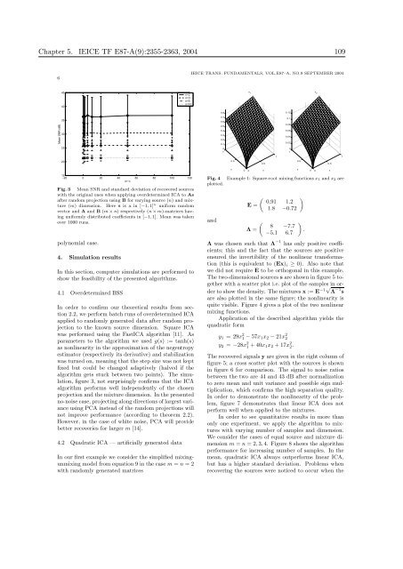
Fig. 4 Example 1: Square-root mixing functions x1 and x2 are
plotted.
and
0.12
0.1
0.08
0.06
0.04
0.02
0
1
0.5
� �
0.91 1.2
E =
1.8 −0.72
� �
8 −7.7
Λ =
.
−5.1 6.7
Λ was chosen such that Λ −1 has only positive coefficients;
this and the fact that the sources are positive
ensured the invertibility of the nonlinear transformation
(this is equivalent to (Ex)i ≥ 0). Also note that
we did not require E to be orthogonal in this example.
The two-dimensional sources s are shown in figure 5 together
with a scatter plot i.e. plot of the samples in order
to show the density. The mixtures x := E −1√ Λ −1 s
are also plotted in the same figure; the nonlinearity is
quite visible. Figure 4 gives a plot of the two nonlinear
mixing functions.
Application of the described algorithm yields the
quadratic form
y1 = 29x 2 1 − 57x1x2 − 21x 2 2
y2 = −28x 2 1 + 40x1x2 + 17x 2 2.
The recovered signals y are given in the right column of
figure 5; a cross scatter plot with the sources is shown
in figure 6 for comparison. The signal to noise ratios
between the two are 44 and 43 dB after normalization
to zero mean and unit variance and possible sign multiplication,
which confirms the high separation quality.
In order to demonstrate the nonlinearity of the problem,
figure 7 demonstrates that linear ICA does not
perform well when applied to the mixtures.
In order to see quantitative results in more than
only one experiment, we apply the algorithm to mixtures
with varying number of samples and dimension.
We consider the cases of equal source and mixture dimension
m = n = 2, 3, 4. Figure 8 shows the algorithm
performance for increasing number of samples. In the
mean, quadratic ICA always outperforms linear ICA,
but has a higher standard deviation. Problems when
recovering the sources were noticed to occur when the
y
x 2
0.5
x
1