

Mathematics in Independent Component Analysis
Mathematics in Independent Component Analysis
Mathematics in Independent Component Analysis

You also want an ePaper? Increase the reach of your titles
YUMPU automatically turns print PDFs into web optimized ePapers that Google loves.
126 Chapter 7. Proc. ISCAS 2005, pages 5878-5881<br />
1<br />
0<br />
−1<br />
0 100 200 300 400 500 600 700 800 900 1000<br />
3<br />
2<br />
1<br />
0<br />
0 100 200 300 400 500 600 700 800 900 1000<br />
1<br />
0<br />
−1<br />
0 100 200 300 400 500 600 700 800 900 1000<br />
3<br />
2<br />
1<br />
0<br />
0 100 200 300 400 500 600 700 800 900 1000<br />
Fig. 2. Simulation, 4-dimensional 2-<strong>in</strong>dependent sources. Clearly the first<br />
and the second respectively the third and the fourth signal are dependent.<br />
B. Simulations<br />
We will discuss algorithm performance when applied to a<br />
4-dimensional 2-<strong>in</strong>dependent toy signal. In order to see the<br />
performance of both MSOBI and MHICA we generate 2<strong>in</strong>dependent<br />
sources with non-trivial autocorrelations. For this<br />
we use two <strong>in</strong>dependent generat<strong>in</strong>g signals, a s<strong>in</strong>usoid and a<br />
sawtooth given by<br />
z(t) := (s<strong>in</strong>(0.1 t), 2⌊0.007 t +0.5⌋−1) ⊤<br />
for discrete time steps t =1, 2,...,1000. We thus generated<br />
sources<br />
s(t) :=(z1(t), exp(z1(t)),z2(t), (z2(t)+0.5) 2 ) ⊤ ,<br />
which are plotted <strong>in</strong> figure 2. Their covariance is<br />
�<br />
Cov(s) =<br />
� 0.50 0.57 0.01 0.01<br />
0.57 0.68 0.01 0.01<br />
0.01 0.01 0.33 0.33<br />
0.01 0.01 0.33 0.42<br />
so <strong>in</strong>deed s is not fully <strong>in</strong>dependent.<br />
s is mixed us<strong>in</strong>g a 4 × 4 matrix A with entries uniformly<br />
drawn out of [−1, 1], and comparisons are made over 100<br />
Monte-Carlo runs. We compare the two algorithms MSOBI<br />
(with 10 autocorrelation matrices) and MHICA (us<strong>in</strong>g 50<br />
Hessians) with the ICA algorithms JADE and fastICA, where<br />
<strong>in</strong> the latter both the deflation and the symmetric approach<br />
was used. For each run we calculate the performance <strong>in</strong>dex<br />
E (2) ( Â−1 A) of the product of the mix<strong>in</strong>g and the estimated<br />
separat<strong>in</strong>g matrix. S<strong>in</strong>ce the one-dimensional ICA algorithms<br />
are unable to use the group structure, for these we take the<br />
m<strong>in</strong>imum of the <strong>in</strong>dex calculated over all row permutations of<br />
 −1 A.<br />
Figure 3 displays the result of the comparison. Clearly<br />
MHICA and MSOBI perform very well on this data, and<br />
MSOBI furthermore gives very robust estimates with the same<br />
error and negligibly small variance. JADE cannot separate<br />
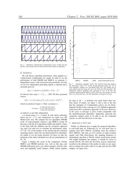
performance <strong>in</strong>dex E (2) ( Â−1 A)<br />
MHICA MSOBI JADE fastICA(defl)fastICA(sym)<br />
Fig. 3. Simulation, algorithm results. This notched boxed plot displays<br />
the performance <strong>in</strong>dex E (2) of the mix<strong>in</strong>g-separat<strong>in</strong>g matrix Â−1 A of<br />
each algorithm, sampled over 100 Monte-Carlo runs. The middle l<strong>in</strong>e of<br />
each column gives the mean, the boxes the 25th and 75th percentile. The<br />
deflationary fastICA algorithm only converged <strong>in</strong> 12% of all runs, the<br />
symmetric-approach based fastICA <strong>in</strong> 89% of all cases; the statistics are only<br />
given over successful runs. All other algorithms converged <strong>in</strong> all runs.<br />
the data at all — it performs not much better than random<br />
choice of matrix, see figure 1; this is due to the fact<br />
that the cumulants of k-<strong>in</strong>dependent sources are not blockdiagonal.<br />
FastICA only converges <strong>in</strong> 12% (deflation approach)<br />
respectively 89% (symmetric approach) of all cases. However,<br />
<strong>in</strong> the cases it converges it gives results comparable with<br />
the multidimensional algorithms. Apparently, especially the<br />
symmetric method seems to be able to use the weakened<br />
statistics to still f<strong>in</strong>d directions <strong>in</strong> the data.<br />
C. Application to ECG data<br />
F<strong>in</strong>ally we illustrate how to apply the proposed algorithms<br />
to real-world data set. Follow<strong>in</strong>g [1], we will show how to<br />
separate fetal ECG (FECG) record<strong>in</strong>gs from the mother’s<br />
ECG (MECG). The data set [13] consists of eight recorded<br />
signals with 2500 observations; the sampl<strong>in</strong>g frequency is<br />
mislead<strong>in</strong>gly specified as 500 Hz (which would mean around<br />
168 mother heartbeats per m<strong>in</strong>ute), it should be closer to<br />
around 250 Hz. We select the first three sensors cutaneously<br />
recorded on the abdomen of the mother. In order to save space<br />
and to compare the results with [1] we plot only the first 1000<br />
samples, see figure 4(a).


