- Page 2 and 3:
PERCEPTUAL COHERENCE
- Page 4 and 5:
Perceptual Coherence Hearing and Se
- Page 6 and 7:
To My Family, My Parents, and the B
- Page 8 and 9:
Preface The purpose of this book is
- Page 10 and 11:
Preface ix intertwined with my own
- Page 12 and 13:
Contents 1. Basic Concepts 3 2. Tra
- Page 14 and 15:
PERCEPTUAL COHERENCE
- Page 16 and 17:
1 Basic Concepts In the beginning G
- Page 18 and 19:
Basic Concepts 5 sources moving in
- Page 20 and 21:
even though its appearance changes.
- Page 22 and 23:
sources. A single sound source is t
- Page 24 and 25:
straight line parallel to the actua
- Page 26 and 27:
continuous sound. The correspondenc
- Page 28 and 29:
Basic Concepts 15 overall uncertain
- Page 30 and 31:
problem. The “snapshots” in spa
- Page 32 and 33:
segments at different orientations.
- Page 34 and 35:
in amplitude across time (analogous
- Page 36 and 37:
Basic Concepts 23 visual experience
- Page 38 and 39:
we would expect the correlation to
- Page 40 and 41:
Transformation of Sensory Informati
- Page 42 and 43:
Transformation of Sensory Informati
- Page 44 and 45:
Table 2.1 Derivation of the Recepti
- Page 46 and 47:
Transformation of Sensory Informati
- Page 48 and 49:
Transformation of Sensory Informati
- Page 50 and 51:
Transformation of Sensory Informati
- Page 52 and 53:
Transformation of Sensory Informati
- Page 54 and 55:
Transformation of Sensory Informati
- Page 56 and 57:
Transformation of Sensory Informati
- Page 58 and 59:
Figure 2.7. Continued
- Page 60 and 61:
Transformation of Sensory Informati
- Page 62 and 63:
Transformation of Sensory Informati
- Page 64 and 65:
Transformation of Sensory Informati
- Page 66 and 67:
Transformation of Sensory Informati
- Page 68 and 69:
Transformation of Sensory Informati
- Page 70 and 71:
Transformation of Sensory Informati
- Page 72 and 73:
Transformation of Sensory Informati
- Page 74 and 75:
Transformation of Sensory Informati
- Page 76 and 77:
Transformation of Sensory Informati
- Page 78 and 79:
Transformation of Sensory Informati
- Page 80 and 81:
Transformation of Sensory Informati
- Page 82 and 83:
Transformation of Sensory Informati
- Page 84 and 85:
Transformation of Sensory Informati
- Page 86 and 87:
Transformation of Sensory Informati
- Page 88 and 89:
Transformation of Sensory Informati
- Page 90 and 91:
Transformation of Sensory Informati
- Page 92 and 93:
Transformation of Sensory Informati
- Page 94 and 95:
Transformation of Sensory Informati
- Page 96 and 97:
Transformation of Sensory Informati
- Page 98 and 99:
Transformation of Sensory Informati
- Page 100 and 101:
Transformation of Sensory Informati
- Page 102 and 103:
Transformation of Sensory Informati
- Page 104 and 105:
Transformation of Sensory Informati
- Page 106 and 107:
Transformation of Sensory Informati
- Page 108 and 109:
Transformation of Sensory Informati
- Page 110 and 111:
3 Characteristics of Auditory and V
- Page 112 and 113:
Information =−Σ. Pr(x i ) log 2
- Page 114 and 115:
Characteristics of Auditory and Vis
- Page 116 and 117:
Characteristics of Auditory and Vis
- Page 118 and 119: Characteristics of Auditory and Vis
- Page 120 and 121: Characteristics of Auditory and Vis
- Page 122 and 123: Characteristics of Auditory and Vis
- Page 124 and 125: Characteristics of Auditory and Vis
- Page 126 and 127: valleys” that support the high-fr
- Page 128 and 129: Characteristics of Auditory and Vis
- Page 130 and 131: Characteristics of Auditory and Vis
- Page 132 and 133: Phase Relationships and Power Laws
- Page 134 and 135: systems to be. One possibility woul
- Page 136 and 137: Characteristics of Auditory and Vis
- Page 138 and 139: are most active, relatively large c
- Page 140 and 141: (see figure 2.2 based on the Differ
- Page 142 and 143: Characteristics of Auditory and Vis
- Page 144 and 145: epresenting these naturally occurri
- Page 146 and 147: Characteristics of Auditory and Vis
- Page 148 and 149: Characteristics of Auditory and Vis
- Page 150 and 151: found in V1. Even though the filter
- Page 152 and 153: Characteristics of Auditory and Vis
- Page 154 and 155: Figure 3.14. The independent compon
- Page 156 and 157: Characteristics of Auditory and Vis
- Page 158 and 159: Characteristics of Auditory and Vis
- Page 160 and 161: specific persons or objects (e.g.,
- Page 162 and 163: amplitudes of each picture and foun
- Page 164 and 165: 4 The Transition Between Noise (Dis
- Page 166 and 167: more cortical levels. For example,
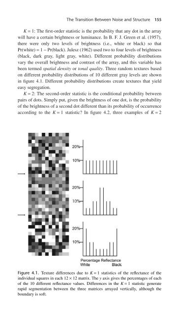
- Page 170 and 171: The Transition Between Noise and St
- Page 172 and 173: The Transition Between Noise and St
- Page 174 and 175: The Transition Between Noise and St
- Page 176 and 177: about poorer performance by creatin
- Page 178 and 179: Figure 4.8. Continued The Transitio
- Page 180 and 181: Surface Textures Visual Glass Patte
- Page 182 and 183: The Transition Between Noise and St
- Page 184 and 185: Figure 4.11. Continued The Transiti
- Page 186 and 187: (A) (B) (C) The Transition Between
- Page 188 and 189: The Transition Between Noise and St
- Page 190 and 191: The Transition Between Noise and St
- Page 192 and 193: The Transition Between Noise and St
- Page 194 and 195: The Transition Between Noise and St
- Page 196 and 197: The Transition Between Noise and St
- Page 198 and 199: (A) (B) Warbleness The Transition B
- Page 200 and 201: The Transition Between Noise and St
- Page 202 and 203: The Transition Between Noise and St
- Page 204 and 205: The Transition Between Noise and St
- Page 206 and 207: 2000 Hz with a single action potent
- Page 208 and 209: The same problem of the multiplicit
- Page 210 and 211: order to create the appearance of s
- Page 212 and 213: Perception of Motion 199 Figure 5.2
- Page 214 and 215: Perception of Motion 201 Figure 5.3
- Page 216 and 217: Perception of Motion 203 together.
- Page 218 and 219:
Perception of Motion 205 (The two f
- Page 220 and 221:
again, two perceptions can result a
- Page 222 and 223:
Perception of Motion 209 Figure 5.6
- Page 224 and 225:
Perception of Motion 211 notes of t
- Page 226 and 227:
Perception of Motion 213 Braddick (
- Page 228 and 229:
larger arrays and Baddeley and Tirp
- Page 230 and 231:
Perception of Motion 217 the judgme
- Page 232 and 233:
Perception of Motion 219 one color
- Page 234 and 235:
To review, neurons sensitive to mot
- Page 236 and 237:
Transparency aftereffects do occur
- Page 238 and 239:
Perception of Motion 225 stimuli, t
- Page 240 and 241:
Perception of Motion 227 Figure 5.1
- Page 242 and 243:
Perception of Motion 229 Figure 5.1
- Page 244 and 245:
Perception of Motion 231 perception
- Page 246 and 247:
Perception of Motion 233 Figure 5.1
- Page 248 and 249:
Perception of Motion 235 Figure 5.1
- Page 250 and 251:
Perception of Motion 237 same direc
- Page 252 and 253:
Time 1, Tone 1 is turned off, at Ti
- Page 254 and 255:
6 Gain Control and External and Int
- Page 256 and 257:
a signal-to-noise ratio), and Barlo
- Page 258 and 259:
Gain Control and External and Inter
- Page 260 and 261:
Gain Control and External and Inter
- Page 262 and 263:
Gain Control and External and Inter
- Page 264 and 265:
Suppose we have a background that h
- Page 266 and 267:
Gain Control and External and Inter
- Page 268 and 269:
Gain Control and External and Inter
- Page 270 and 271:
R Gain Control and External and Int
- Page 272 and 273:
Makous (1997) pointed out how diffi
- Page 274 and 275:
contrast that defines the boundarie
- Page 276 and 277:
per Second Figure 6.10. Continued G
- Page 278 and 279:
Gain Control and External and Inter
- Page 280 and 281:
ane was linear, the higher sound pr
- Page 282 and 283:
(C. D. Geisler, 1998; C. D. Geisler
- Page 284 and 285:
Gain Control and External and Inter
- Page 286 and 287:
noise visual field. 4 The S + N inp
- Page 288 and 289:
B. Murray, Bennett, and Sekular (20
- Page 290 and 291:
The authors proposed that the four
- Page 292 and 293:
Gain Control and External and Inter
- Page 294 and 295:
Efficiency and Noise in Auditory Pr
- Page 296 and 297:
etween samples). Spiegel and Green
- Page 298 and 299:
Gain Control and External and Inter
- Page 300 and 301:
Gain Control and External and Inter
- Page 302 and 303:
Gain Control and External and Inter
- Page 304 and 305:
In sum, the masking release is grea
- Page 306 and 307:
The Perception of Quality: Visual C
- Page 308 and 309:
The Perception of Quality: Visual C
- Page 310 and 311:
Visual Worlds Modeling the Light Re
- Page 312 and 313:
Indirect Illumination Causing Specu
- Page 314 and 315:
of an object but also require the c
- Page 316 and 317:
assumed, so that the surface irradi
- Page 318 and 319:
The Perception of Quality: Visual C
- Page 320 and 321:
The Perception of Quality: Visual C
- Page 322 and 323:
Relative Power of Basis Functions S
- Page 324 and 325:
The Perception of Quality: Visual C
- Page 326 and 327:
that the reflectance of the test co
- Page 328 and 329:
The Perception of Quality: Visual C
- Page 330 and 331:
amount of light transmitted through
- Page 332 and 333:
light reflected by all surfaces in
- Page 334 and 335:
The Perception of Quality: Visual C
- Page 336 and 337:
The Perception of Quality: Visual C
- Page 338 and 339:
The Perception of Quality: Visual C
- Page 340 and 341:
The Perception of Quality: Visual C
- Page 342 and 343:
magenta to white). Then Bloj et al.
- Page 344 and 345:
Why is there opponent processing? O
- Page 346 and 347:
8 The Perception of Quality: Audito
- Page 348 and 349:
exists at several levels: (a) descr
- Page 350 and 351:
The Perception of Quality: Auditory
- Page 352 and 353:
mode is proportional to the relativ
- Page 354 and 355:
The Perception of Quality: Auditory
- Page 356 and 357:
The overall result is that the rela
- Page 358 and 359:
obvious. The tension on the vocal c
- Page 360 and 361:
The Perception of Quality: Auditory
- Page 362 and 363:
(termed the amplitude envelopes) ar
- Page 364 and 365:
The Perception of Quality: Auditory
- Page 366 and 367:
The Perception of Quality: Auditory
- Page 368 and 369:
obviously misplaced). The majority
- Page 370 and 371:
The Perception of Quality: Auditory
- Page 372 and 373:
Pastore (1991) investigated whether
- Page 374 and 375:
experience. Erickson (2003) found t
- Page 376 and 377:
Rhythmic patterning usually gives i
- Page 378 and 379:
The Perception of Quality: Auditory
- Page 380 and 381:
Let me summarize at this point. The
- Page 382 and 383:
The Perception of Quality: Auditory
- Page 384 and 385:
the oddball note to be the one most
- Page 386 and 387:
9 Auditory and Visual Segmentation
- Page 388 and 389:
Auditory and Visual Segmentation 37
- Page 390 and 391:
Auditory and Visual Segmentation 37
- Page 392 and 393:
Auditory and Visual Segmentation 37
- Page 394 and 395:
processes (e.g., basilar membrane v
- Page 396 and 397:
same time, the difficulty of detect
- Page 398 and 399:
elease (discussed in chapter 6) dem
- Page 400 and 401:
Auditory and Visual Segmentation 38
- Page 402 and 403:
(A) Target Rhythm Target + Masking
- Page 404 and 405:
to grouping by perceived position d
- Page 406 and 407:
4. Convexity: Convex figures usuall
- Page 408 and 409:
Auditory and Visual Segmentation 39
- Page 410 and 411:
Auditory and Visual Segmentation 39
- Page 412 and 413:
Auditory and Visual Segmentation 39
- Page 414 and 415:
Auditory and Visual Segmentation 40
- Page 416 and 417:
filter inferred from the background
- Page 418 and 419:
Auditory and Visual Segmentation 40
- Page 420 and 421:
Jackson (1953) found that the sound
- Page 422 and 423:
Auditory and Visual Segmentation 40
- Page 424 and 425:
Auditory and Visual Segmentation 41
- Page 426 and 427:
Auditory and Visual Segmentation 41
- Page 428 and 429:
a speaking face is located in front
- Page 430 and 431:
was high, then the resolution of th
- Page 432 and 433:
Listeners were more likely to repor
- Page 434 and 435:
10 Summing Up Perceiving is the con
- Page 436 and 437:
Summing Up 423 course of the stimul
- Page 438 and 439:
References Adelson, E. H. (1982). S
- Page 440 and 441:
References 427 Bermant, R. I., & We
- Page 442 and 443:
References 429 Crawford, B. H. (194
- Page 444 and 445:
References 431 Feldman, J., & Singh
- Page 446 and 447:
References 433 and male voices in t
- Page 448 and 449:
References 435 Isabelle, S. K., & C
- Page 450 and 451:
References 437 Laughlin, S. B. (200
- Page 452 and 453:
References 439 McAdams, S., Winsber
- Page 454 and 455:
References 441 Pittinger, J. B., Sh
- Page 456 and 457:
References 443 Shamma, S. (2001). O
- Page 458 and 459:
References 445 Troost, J. M. (1998)
- Page 460 and 461:
References 447 Welch, R. B. (1999).
- Page 462 and 463:
Index Boldfaced entries refer to ci
- Page 464 and 465:
Barbour, D. L., 83, 367, 426 Barlow
- Page 466 and 467:
Color reflectance 1/f c amplitude f
- Page 468 and 469:
Figure-ground auditory, 373, 421 in
- Page 470 and 471:
Hallikainen, J., 304, 440 Handel, S
- Page 472 and 473:
K-order statistics. See Visual text
- Page 474 and 475:
separation of things, 5 See also Pe
- Page 476 and 477:
Recanzone, G. H., 409-412, 441, 443
- Page 478 and 479:
Stream segregation default assumpti
- Page 480 and 481:
vibration frequencies of air masses
- Page 482:
Wavelet analysis. See Sparse coding