Note de curs - Departamentul Automatica, Calculatoare si ...

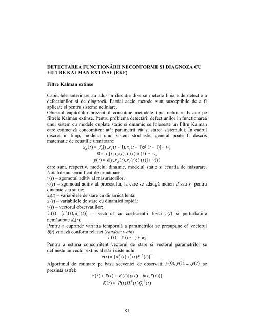
DETECTAREA FUNCTIONǍRII NECONFORME SI DIAGNOZA CU
FILTRE KALMAN EXTINSE (EKF)
Filtre Kalman extinse
Capitolele anterioare au adus în discutie diverse metode liniare de detectie a
defectiunilor si de diagnozǎ. Partial acele metode sunt susceptibile de a fi
aplicate si pentru sisteme neliniare.
Obiectul capitolului prezent îl constituie metodele tipic neliniare bazate pe
filtrele Kalman extinse. Pentru problema detectǎrii defectiunilor în functionarea
unui sistem cu modele cuplate static si dinamic se foloseste un filtru Kalman
care estimeazǎ concomitent atât parametrii cât si starea sistemului. În cadrul
discret în timp, modelul unui sistem stochastic general poate fi descris
matematic de ecuatiile urmǎtoare:
xd ( t) = f
d[ t, xd ( t − 1), xs( t − 1); θ ( t − 1)]
+ wd
0 = f
s[ t, xd ( t), xs( t); θ ( t)]
+ ws
y( t) = h[ t, xd
( t), xs( t); θ ( t)] + v( t)
care sunt, respectiv, modelul dinamic, modelul static si ecuatia de mǎsurare.
Notatiile au semnificatiile urmǎtoare:
v(t) – zgomotul aditiv al mǎsurǎtorilor;
w(t) – zgomotul aditiv al procesului, la care se adaugǎ indicii d sau s pentru
dinamic sau static;
x d (t) – variabilele de stare cu dinamicǎ lentǎ;
x s (t) – variabilele de stare cu dinamicǎ rapidǎ;
y(t) – vectorul observatiilor;
θ ( t) [ c T T
= ( t), du
( t)]
– vectorul cu coeficientii fizici c(t) si perturbatiile
nemǎsurate d u (t).
Pentru a cuprinde variatia temporalǎ a parametrilor se presupune cǎ vectorul
θ(t) variazǎ conform relatiei (random walk)
θ ( t) = θ ( t − 1)
+ wθ
Pentru a estima concomitent vectorul de stare si vectorul parametrilor se
defineste un vector extins al stǎrii sistemului
T T T T
z ( t)
= [ xd
( t)
xs
( t)
θ ( t)]
Algoritmul de estimare pe baza secventei de observatii y( 0), y( 1 ),..., y( t)
se
prezintǎ astfel:
z( t) = z( t) + K( t)[ y( t) − h( t, z( t))]
T
− 1
K( t) = P( t) H ( t) Q ( t)
v
81