Project Cyclops, A Design... - Department of Earth and Planetary ...

We conclude that none of the above alternatives is
attractive, and the best way to avoid chromatic aberration
in a delay line imager is to image at the original
band, or near it.
If we wish to have m image points and if the n
antennas in our array were scattered at random points,
we would require mn cables to make all the connections
in the imager. For n = 1000 and m = 4000 we need 4
million cables. However, if both the antennas and the
image points are in regular lattice patterns, this number
can be reduced by performing the transformation in two
steps as allowed by equation (38).
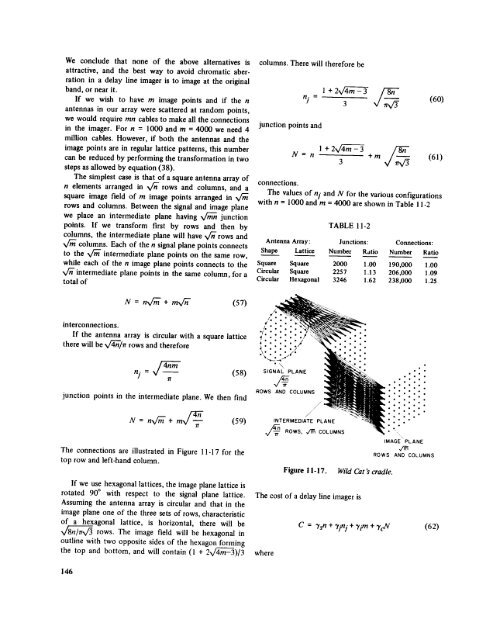
The simplest case is that of a square antenna array of
n elements arranged in _ rows and colunms, and a
square image field of m image points arranged in V_
rows and columns. Between the signal and image plane
we place an intermediate plane having _ junction
points. If we transform first by rows and then by
columns, the intermediate plane will have V_" rows and
V_ columns. Each of the n signal plane points connects
to the V_" intermediate plane points on the same row,
while each of the n image plane points connects to the
intermediate plane points in the same column, for a
total of
columns. There will therefore be
junction points and
connections.
1+2v - -3
n]- 3
(60)
N = n 1+2 + m (61)
3
The values of n] and N for the various configurations
with n = 1000 and m = 4000 are shown in Table 11-2
TABLE 11-2
Antenna Array: Junctions: Connections:
Shape Lattice Number Ratio Number Ratio
Square Square 2000 1.00 190,000 1.00
Circular Square 2257 1.13 206,000 1.09
Circular Hexagonal 3246 1.62 238,000 1.25
N = nv_ + mVrff" (57)
interconnections.
If the antenna array is circular with a square lattice
there will be x/r_"/lr rows and therefore
= (58)
,/o • • °
* o "/I I. • I I
•': 2:-X/"
• x
\,
SIGNAL PLANE
junction points in the intermediate plane. We then find
ROWS AND COLUMNS
/
/
(59)
INTERMEDIATE
PLANE
•v_ ROWS, _ COLUMNS
The connections are illustrated in Figure 11-17 for the
top row and left-hand column.
If we use hexagonal lattices, the image plane lattice is
rotated 90 ° with respect to the signal plane lattice.
Assuming the antenna array is circular and that in the
image plane one of the three sets of rows, characteristic
of a hexagonal lattice, is horizontal, there will be
_x/'3 rows. The image field will be hexagonal in
outline with two opposite sides of the hexagon forming
the top and bottom, and will contain (i + 2_)/3
The cost
where
Figure 11-17. Wild Cat's cradle.
of a delay line imager is
C = "ysn+ "y/n/+"yim + VcN (62)
146