Project Cyclops, A Design... - Department of Earth and Planetary ...

where0ma x is the maximum value of 0 we can allow
(see Figure 11-18) and 6ma x is the corresponding value
of 6 (see Figure 11-16). We can consider using electromagnetic
waves because 0ma x can be much greater than
5ma x and therefore the scale factor o can be very small.
Let us assume we wish to image over the tuning range
from l to 3 GHz. Then kmax = 0.3 m. If we choose
s = 2_.ma x = 0.6 m, then for a 1000-element array
a _ 10 m. We can easily space the receiving antennas at s/2
so we choose b/a = 1 in equation (66) and find £ _ 40 m.
Whereas the array dimensions in acoustic imaging were
very small, the dimensions involved in microwave imaging
are larger than we would like, but not impractically
large.
A great advantage of microwave imaging over delay
line or acoustic imaging is that we can vary the image
size by changing £, thus allowing us to match the useful
field size to the image array size as we vary the operating
frequency. At 3 GHz, for example, we can use the same
arrays as in the above example but increase _ to 120 m.
But to realize this advantage we must be able to keep the
image focused as I_is changed.
One way to focus a microwave imager is with an
artificial dielectric lens in front of the signal plane and a
similar lens in front of the image plane to flatten the
field. This allows both arrays to be plane, but requires
several pairs of lenses to cover the frequency range. The
cost and practicality of artificial dielectric lenses 20 m or
more in diameter have not been evaluated.
The use of concave arrays causes great mechanical
complications since the iadii of curvature must be
changed as the separation is changed. The following
possibilities were explored
aberrations within tolerable limits over a plane image
surface.
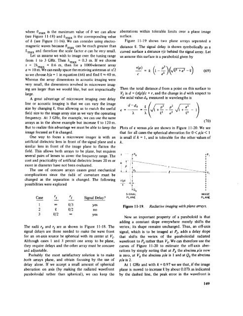
Figure 11-19 shows two plane arrays separated a
distance _. The signal delay is shown symbolically as a
curved surface a distance z/c behind the signal array. Let
us assume this surface is a paraboloid given by
"r_) c - k (1 _ _-)(X/_+a p2 2- _) (69)
Then the total distance d from a point on this surface to
Vi is d = (r(p)/c + r, and the change in d with respect to
the axial value do measured in wavelengths is
__ =__ -i--- --m +-- --
X ;_ _2 as _2
(70)
Plots of e versus p[a are shown in Figure 11-20. We see
that for all cases the spherical aberration for 0 < p/a < 1
is small if k = 1, and is tolerable for the other values of
k.
a, /,""
I p ,+
C
I_IQ s
r
I
Vi
Case rs ri Signal Delay?
SIGNAL
PLANE
IMAGE
PLANE
1 oo £/3 yes
2 _ _/2 no
3 _/2 oo yes
The radii rs and ri are as shown in Figure 11-18. The
signal delays are those needed to make the wave front
for an on-axis source be spherical with its center at Vi.
Although cases 1 and 3 permit one array to be plane,
they require delays and the other array must be concave
and adjustable.
Probably the most satisfactory solution is to make
both arrays plane, and obtain focusing by the use of
delay alone. If we accept a small amount of spherical
aberration on axis (by making the radiated wavefront
paraboloidal rather than spherical), we can keep the
Figure 11-19. Radiative imaging with plane arrays.
Now an important property of a paraboloid is that
adding a constant slope everywhere merely shifts the
vertex; its shape remains unchanged. Thus, an off-axis
signal, which is to be imaged at Pi, adds a delay slope
that shifts the vertex of the paraboloidal radiated
wavefront to Ps rather than V s. We can therefore use the
curves of Figure 11-20 to estimate the off-axis aberrations
by simply noting that at Ps the abscissa #/a now
is zero, at Vs the abscissa p/a is 1 and at Qs the abscissa
p/a is 2.
At 1 GHz and with k = 0.97 we see that, if the image
plane is moved to increase £ by about 0.077_ as indicated
by the dashed line, the peak error in the wavefront is
149