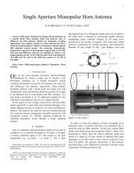
PPKE ITK PhD and MPhil Thesis Classes
PPKE ITK PhD and MPhil Thesis Classes
PPKE ITK PhD and MPhil Thesis Classes

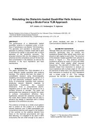
Create successful ePaper yourself
Turn your PDF publications into a flip-book with our unique Google optimized e-Paper software.
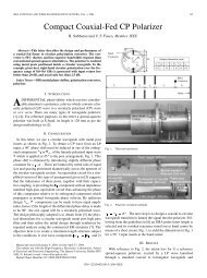
50<br />
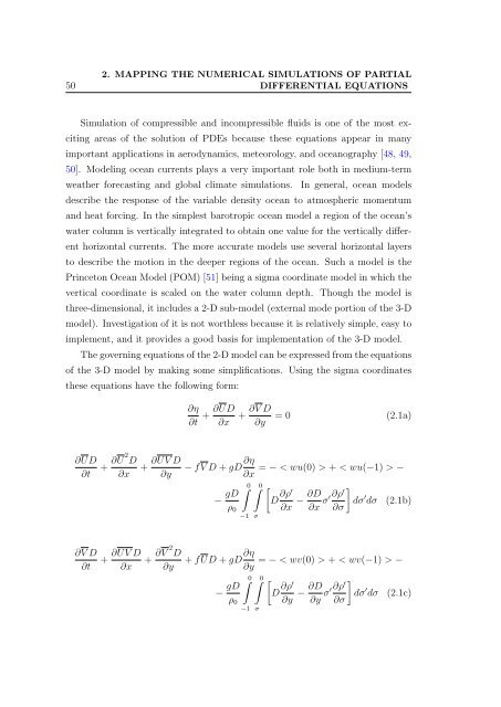
2. MAPPING THE NUMERICAL SIMULATIONS OF PARTIAL<br />
DIFFERENTIAL EQUATIONS<br />
Simulation of compressible <strong>and</strong> incompressible fluids is one of the most exciting<br />
areas of the solution of PDEs because these equations appear in many<br />
important applications in aerodynamics, meteorology, <strong>and</strong> oceanography [48, 49,<br />
50]. Modeling ocean currents plays a very important role both in medium-term<br />
weather forecasting <strong>and</strong> global climate simulations.<br />
In general, ocean models<br />
describe the response of the variable density ocean to atmospheric momentum<br />
<strong>and</strong> heat forcing. In the simplest barotropic ocean model a region of the ocean’s<br />
water column is vertically integrated to obtain one value for the vertically different<br />
horizontal currents. The more accurate models use several horizontal layers<br />
to describe the motion in the deeper regions of the ocean. Such a model is the<br />
Princeton Ocean Model (POM) [51] being a sigma coordinate model in which the<br />
vertical coordinate is scaled on the water column depth. Though the model is<br />
three-dimensional, it includes a 2-D sub-model (external mode portion of the 3-D<br />
model). Investigation of it is not worthless because it is relatively simple, easy to<br />
implement, <strong>and</strong> it provides a good basis for implementation of the 3-D model.<br />
The governing equations of the 2-D model can be expressed from the equations<br />
of the 3-D model by making some simplifications. Using the sigma coordinates<br />
these equations have the following form:<br />
∂η<br />
∂t + ∂UD<br />
∂x<br />
+ ∂V D<br />
∂y<br />
= 0 (2.1a)<br />
∂UD<br />
∂t<br />
+ ∂U 2 D<br />
∂x<br />
+ ∂UV D<br />
∂y<br />
− fV D + gD ∂η = − < wu(0) > + < wu(−1) > −<br />
∂x<br />
− gD ∫0<br />
∫ 0 [D ∂ρ′<br />
ρ 0 ∂x − ∂D ]<br />
∂ρ′<br />
σ′ dσ ′ dσ (2.1b)<br />
∂x ∂σ<br />
−1<br />
σ<br />
∂V D<br />
∂t<br />
+ ∂UV D<br />
∂x<br />
+ ∂V 2 D<br />
∂y<br />
+ fUD + gD ∂η = − < wv(0) > + < wv(−1) > −<br />
∂y<br />
− gD ∫0<br />
∫ 0 [D ∂ρ′<br />
ρ 0 ∂y − ∂D ]<br />
∂ρ′<br />
σ′ dσ ′ dσ (2.1c)<br />
∂y ∂σ<br />
−1<br />
σ


![optika tervezés [Kompatibilitási mód] - Ez itt...](https://img.yumpu.com/45881475/1/190x146/optika-tervezacs-kompatibilitasi-mad-ez-itt.jpg?quality=85)