PPKE ITK PhD and MPhil Thesis Classes

More documents

Recommendations

Info

54 2. MAPPING THE NUMERICAL SIMULATIONS OF PARTIAL DIFFERENTIAL EQUATIONS On the other hand, the development time of an optimized software solution is much shorter than designing a reconfigurable architecture [56][57], however, the computational efficiency is smaller in terms of area and power. Namely on FPGAs we can make a more specific structure for the CFD with better performance in terms of the area and dissipation with a variable accuracy considering to use it in real life applications. 2.3.2 Fluid Flows A wide range of industrial processes and scientific phenomena involve gas or fluids flows over complex obstacles. In engineering applications the temporal evolution of non-ideal, compressible fluids is quite often modeled by Navier-Stokes [58, 59] equations. It is based on the fundamental laws of mass-, momentum- and energy conservation, extended by the dissipative effects of viscosity, diffusion and heat conduction. By neglecting all the above non-ideal processes, and assuming adiabatic variations, we obtain the Euler equations [60, 61], describing the dynamics of dissipation-free, inviscid, compressible fluids. The equations, a coupled set of nonlinear hyperbolic partial differential equations, in conservative form expressed as ∂ (ρv) ∂t ∂E ∂t ∂ρ ∂t + ∇ · (ρv) = 0 (2.2) ) + ∇ · (ρvv + Îp = 0 (2.3) + ∇ · ((E + p)v) = 0, (2.4) where t denotes time, ∇ is the Nabla operator, ρ is the density, u, v are the x- and y-components of velocity vector v, respectively, p is the pressure of the fluid, Î is the identity matrix, and E is the total energy density defined as E = p γ − 1 + 1 ρv · v, (2.5) 2 where γ is the ratio of specific heats. It is convenient to merge (2.2), (2.3) and (2.4) into hyperbolic conservation law form in terms of U = [ρ, ρu, ρv, E] and the
2.3 Computational Fluid Flow Simulation on Body Fitted Mesh Geometry with IBM Cell Broadband Engine and FPGA Architecture 55 flux tensor as ⎛ F = ⎝ ∂U ∂t ρv ρvv + Ip (E + p)v ⎞ ⎠ (2.6) + ∇ · F = 0. (2.7) 2.3.2.1 Discretization of the governing equations Since logically structured arrangement of data is fundamental for the efficient operation of the FPGA based implementations, we consider explicit finite volume discretizations [62] of the governing equations over structured grids employing a simple numerical flux function. Indeed, the corresponding rectangular arrangement of information and the choice of multi-level a temporal integration strategy ensure the continuous flow of data through the CNN-UM architecture. In the followings we recall the basic properties of the mesh geometry, and the details of the considered first- and second-order schemes. 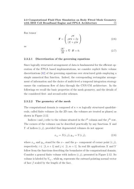2.3.2.2 The geometry of the mesh The computational domain is composed of n × m logically structured quadrilaterals, called finite volumes (in the 2D case, the volumes are treated as planes) as shown in Figure 2.12. Indices i and j refer to the volume situated in the i th column and the j th row. The corners of the volumes can be described practically by any functions X and Y of indices (i, j), provided that degenerated volumes do not appear: x i,j = X(i, j), y i,j = Y (i, j), (2.8) where x i,j and y i,j stand for the x− and the y− component of corner point (i, j), respectively, i ∈ [1, n + 1] and j ∈ [1, m + 1]. In real life applications X and Y follow from the functions describing the boundaries of the computational domain. Consider a general finite volume with indices (i, j), presented in Figure 2.12. Its volume is labeled by V i,j , while n f represents the outward pointing normal vector of face f scaled by the length of the face.
Page 1:
An Optimal Mapping of Numerical Sim
Page 5 and 6:
Acknowledgements It is not so hard
Page 7 and 8:
Contents 1 Introduction 1 1.1 Cellu
Page 9:
CONTENTS iii 4.3.3 Operating Steps
Page 12 and 13:
vi LIST OF FIGURES 2.4 Performance
Page 15:
List of Tables 2.1 Comparison of di
Page 18 and 19:
xii LIST OF ABBREVIATIONS FPE Falco
Page 21 and 22:
Chapter 1 Introduction Due to the r
Page 23 and 24: 3 can be represented in arbitrary t
Page 25 and 26: 1.1 Cellular Neural/Nonlinear Netwo
Page 27 and 28: 1.2 Cellular Neural/Nonlinear Netwo
Page 29 and 30: 1.3 CNN-UM Implementations 9 the Lo
Page 31 and 32: 1.3 CNN-UM Implementations 11 modif
Page 33 and 34: 1.4 Field Programmable Gate Arrays
Page 47 and 48: 1.5 IBM Cell Broadband Engine Archi
Page 55 and 56: Chapter 2 Mapping the Numerical Sim
Page 57 and 58: 2.1 Introduction 37 18 Load instruc
Page 59 and 60: 2.1 Introduction 39 Instruction his
Page 61 and 62: 2.1 Introduction 41 2E+07 1E+07 9E+
Page 63 and 64: 2.1 Introduction 43 Main memory 8 t
Page 65 and 66: 2.1 Introduction 45 6 4.5 3 Speedup
Page 67 and 68: 2.1 Introduction 47 2.50E+07 1.88E+
Page 69 and 70: 2.2 Ocean model and its implementat
Page 71 and 72: 2.2 Ocean model and its implementat
Page 73: 2.3 Computational Fluid Flow Simula
Page 77 and 78: 2.3 Computational Fluid Flow Simula
Page 89 and 90: Chapter 3 Investigating the Precisi
Page 91 and 92: 3.2 Numerical Solutions of the PDEs
Page 93 and 94: 3.3 Testing Methodology 73 In fixed
Page 95 and 96: 3.4 Properties of the Arithmetic Un
Page 97 and 98: 3.4 Properties of the Arithmetic Un
Page 99 and 100: 3.5 Results 79 in the L2 cache of t
Page 101 and 102: 3.5 Results 81 1E-02 1E-03 Error 1E
Page 103 and 104: 3.5 Results 83 arithmetic unit requ
Page 105: 3.6 Conclusion 85 point and the 40
Page 108 and 109: 4. IMPLEMENTING A GLOBAL ANALOGIC P
Page 124 and 125:
4. IMPLEMENTING A GLOBAL ANALOGIC P
Page 126 and 127:
Page 128 and 129:
Page 130 and 131:
110 5. SUMMARY OF NEW SCIENTIFIC RE
Page 132 and 133:
Page 134 and 135:
Page 136 and 137:
Page 138 and 139:
Page 141 and 142:
References The author’s journal p
Page 143 and 144:
5.2 Application of the results 123
Page 145 and 146:
Page 147 and 148:
show all

PPKE ITK PhD and MPhil Thesis Classes

Create successful ePaper yourself

Delete template?

Save as template?