PPKE ITK PhD and MPhil Thesis Classes

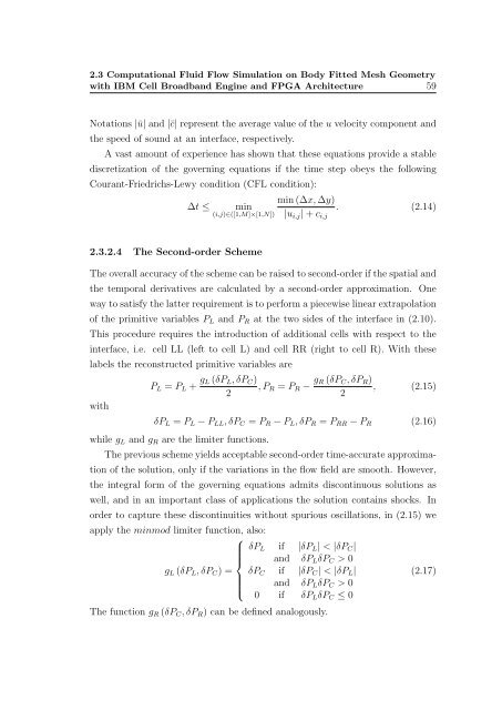
2.3 Computational Fluid Flow Simulation on Body Fitted Mesh Geometry
with IBM Cell Broadband Engine and FPGA Architecture 59
Notations |ū| and |¯c| represent the average value of the u velocity component and
the speed of sound at an interface, respectively.
A vast amount of experience has shown that these equations provide a stable
discretization of the governing equations if the time step obeys the following
Courant-Friedrichs-Lewy condition (CFL condition):
∆t ≤
min (∆x, ∆y)
min
. (2.14)
(i,j)∈([1,M]×[1,N]) |u i,j | + c i,j
2.3.2.4 The Second-order Scheme
The overall accuracy of the scheme can be raised to second-order if the spatial and
the temporal derivatives are calculated by a second-order approximation. One
way to satisfy the latter requirement is to perform a piecewise linear extrapolation
of the primitive variables P L and P R at the two sides of the interface in (2.10).
This procedure requires the introduction of additional cells with respect to the
interface, i.e. cell LL (left to cell L) and cell RR (right to cell R). With these
labels the reconstructed primitive variables are
with
P L = P L + g L (δP L , δP C )
2
, P R = P R − g R (δP C , δP R )
, (2.15)
2
δP L = P L − P LL , δP C = P R − P L , δP R = P RR − P R (2.16)
while g L and g R are the limiter functions.
The previous scheme yields acceptable second-order time-accurate approximation
of the solution, only if the variations in the flow field are smooth. However,
the integral form of the governing equations admits discontinuous solutions as
well, and in an important class of applications the solution contains shocks. In
order to capture these discontinuities without spurious oscillations, in (2.15) we
apply the minmod limiter function, also:
⎧
δP L if |δP L | < |δP C |
⎪⎨ and δP L δP C > 0
g L (δP L , δP C ) = δP C if |δP C | < |δP L |
and δP L δP C > 0
⎪⎩
0 if δP L δP C ≤ 0
The function g R (δP C , δP R ) can be defined analogously.
(2.17)