PPKE ITK PhD and MPhil Thesis Classes

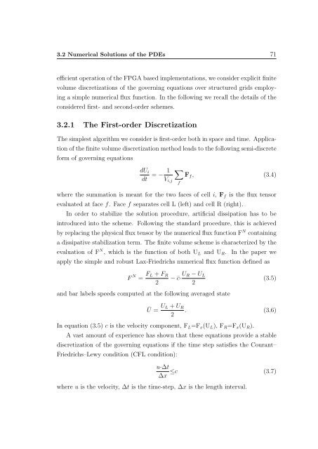
3.2 Numerical Solutions of the PDEs 71
efficient operation of the FPGA based implementations, we consider explicit finite
volume discretizations of the governing equations over structured grids employing
a simple numerical flux function. In the following we recall the details of the
considered first- and second-order schemes.
3.2.1 The First-order Discretization
The simplest algorithm we consider is first-order both in space and time. Application
of the finite volume discretization method leads to the following semi-discrete
form of governing equations
dU i
dt = − 1 ∑
F f , (3.4)
V i,j
where the summation is meant for the two faces of cell i, F f is the flux tensor
evaluated at face f. Face f separates cell L (left) and cell R (right).
In order to stabilize the solution procedure, artificial dissipation has to be
introduced into the scheme. Following the standard procedure, this is achieved
by replacing the physical flux tensor by the numerical flux function F N containing
a dissipative stabilization term. The finite volume scheme is characterized by the
evaluation of F N , which is the function of both U L and U R . In the paper we
apply the simple and robust Lax-Friedrichs numerical flux function defined as
f
F N = F L + F R
2
− ¯c·UR − U L
2
and bar labels speeds computed at the following averaged state
(3.5)
Ū = U L + U R
. (3.6)
2
In equation (3.5) c is the velocity component, F L =F x (U L ), F R =F x (U R ).
A vast amount of experience has shown that these equations provide a stable
discretization of the governing equations if the time step satisfies the Courant–
Friedrichs–Lewy condition (CFL condition):
u·∆t
≤c (3.7)
∆x
where u is the velocity, ∆t is the time-step, ∆x is the length interval.