PPKE ITK PhD and MPhil Thesis Classes

More documents

Recommendations

Info

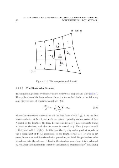
56 2. MAPPING THE NUMERICAL SIMULATIONS OF PARTIAL DIFFERENTIAL EQUATIONS (n+1;m+1) x x n 2 x x x x x (i;j) n 1 x x x n 3 n 4 x x (1;1) Figure 2.12: The computational domain 2.3.2.3 The First-order Scheme The simplest algorithm we consider is first-order both in space and time [56] [57]. The application of the finite volume discretization method leads to the following semi-discrete form of governing equations (2.6) dU i,j dt = − 1 ∑ F f · n f , (2.9) V i,j where the summation is meant for all the four faces of cell (i,j), F f is the flux tensor evaluated at face f, and n f is the outward pointing normal vector of face f scaled by the length of the face. Let us consider face f in a coordinate frame attached to the face, such that its x-axes is normal to f. Face f separates cell L (left) and cell R (right). In this case the F f · n f scalar product equals to the x-component of F(F x ) multiplied by the length of the face (or area in 3D case). In order to stabilize the solution procedure, artificial dissipation has to be introduced into the scheme. Following the standard procedure, this is achieved by replacing the physical flux tensor by the numerical flux function F N containing f
2.3 Computational Fluid Flow Simulation on Body Fitted Mesh Geometry with IBM Cell Broadband Engine and FPGA Architecture 57 the dissipative stabilization term. A finite volume scheme is characterized by the evaluation of F N , which is the function of both U L and U R . Applying the simple and robust Lax-Friedrichs numerical flux function defined as F N = F L + F R 2 − (|ū| + ¯c) U R − U L . (2.10) 2 In the last equation c is the local speed of sound, F L =F x (U L ), F R =F x (U R ) and bar labels speeds computed at the following averaged state Ū = U L + U R . (2.11) 2 The last step concludes the spatial discretization. Finally, the temporal derivative is dicretized by the first-order forward Euler method: dU i,j dt = U n+1 i,j − Ui,j n ∆t , (2.12) where U n i,j is the known value of the state vector at time instant n, U n+1 i,j the unknown value of the state vector at time instant n + 1, and ∆t the time step. By working out the algebra described so far, leads to the following discrete form
Page 1:
An Optimal Mapping of Numerical Sim
Page 5 and 6:
Acknowledgements It is not so hard
Page 7 and 8:
Contents 1 Introduction 1 1.1 Cellu
Page 9:
CONTENTS iii 4.3.3 Operating Steps
Page 12 and 13:
vi LIST OF FIGURES 2.4 Performance
Page 15:
List of Tables 2.1 Comparison of di
Page 18 and 19:
xii LIST OF ABBREVIATIONS FPE Falco
Page 21 and 22:
Chapter 1 Introduction Due to the r
Page 23 and 24:
3 can be represented in arbitrary t
Page 25 and 26: 1.1 Cellular Neural/Nonlinear Netwo
Page 27 and 28: 1.2 Cellular Neural/Nonlinear Netwo
Page 29 and 30: 1.3 CNN-UM Implementations 9 the Lo
Page 31 and 32: 1.3 CNN-UM Implementations 11 modif
Page 33 and 34: 1.4 Field Programmable Gate Arrays
Page 47 and 48: 1.5 IBM Cell Broadband Engine Archi
Page 55 and 56: Chapter 2 Mapping the Numerical Sim
Page 57 and 58: 2.1 Introduction 37 18 Load instruc
Page 59 and 60: 2.1 Introduction 39 Instruction his
Page 61 and 62: 2.1 Introduction 41 2E+07 1E+07 9E+
Page 63 and 64: 2.1 Introduction 43 Main memory 8 t
Page 65 and 66: 2.1 Introduction 45 6 4.5 3 Speedup
Page 67 and 68: 2.1 Introduction 47 2.50E+07 1.88E+
Page 69 and 70: 2.2 Ocean model and its implementat
Page 71 and 72: 2.2 Ocean model and its implementat
Page 73 and 74: 2.3 Computational Fluid Flow Simula
Page 75: 2.3 Computational Fluid Flow Simula
Page 89 and 90: Chapter 3 Investigating the Precisi
Page 91 and 92: 3.2 Numerical Solutions of the PDEs
Page 93 and 94: 3.3 Testing Methodology 73 In fixed
Page 95 and 96: 3.4 Properties of the Arithmetic Un
Page 97 and 98: 3.4 Properties of the Arithmetic Un
Page 99 and 100: 3.5 Results 79 in the L2 cache of t
Page 101 and 102: 3.5 Results 81 1E-02 1E-03 Error 1E
Page 103 and 104: 3.5 Results 83 arithmetic unit requ
Page 105: 3.6 Conclusion 85 point and the 40
Page 108 and 109: 4. IMPLEMENTING A GLOBAL ANALOGIC P
Page 126 and 127:
4. IMPLEMENTING A GLOBAL ANALOGIC P
Page 128 and 129:
4. IMPLEMENTING A GLOBAL ANALOGIC P
Page 130 and 131:
110 5. SUMMARY OF NEW SCIENTIFIC RE
Page 132 and 133:
Page 134 and 135:
Page 136 and 137:
Page 138 and 139:
Page 141 and 142:
References The author’s journal p
Page 143 and 144:
5.2 Application of the results 123
Page 145 and 146:
Page 147 and 148:
show all

PPKE ITK PhD and MPhil Thesis Classes

Create successful ePaper yourself

Delete template?

Save as template?