Download Full Issue in PDF - Academy Publisher

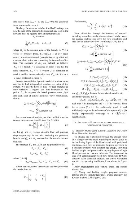
1474 JOURNAL OF COMPUTERS, VOL. 8, NO. 6, JUNE 2013
into node i then e = −1
, and e = 0 if the generator
Qini
is not connected to node i .
Similarly, the network satisfies Kirchhoff's voltage law,
i.e., the sum of the pressure drops around any loop in the
network must be equal to zero, or mathematically
E H
H = 0 or
n
∑
j = 1
E
Hij
H
j
Qini
= 0,
i = 1, , l,
(5)
where H
j
is the pressure drop of the branch j , H is a
vector of pressure drops, E
H
= [ EHij
] is an l × n mesh
matrix, in which each mesh (loop) is formed by a link and
a unique chain in the tree connecting the two nodes of the
link. The elements of E Hij
are defined as follows:
E
Hij
= 1 if branch j is contained in mesh i and has the
same direction, E
Hij
= −1
if branch j is contained in
mesh i and has the opposite direction, E
Hij
= 0 if branch
j is not contained in mesh i .
In order to establish a dynamic model of minimal order,
one has to find independent variables as states of the
system. We take the flows of link (co-tree) branches as
state variables. If regards one time heartbeat as one
period T , decomposes the blood pressure wave f (t)
into each kind of simple harmonic wave combination,
that is:
n
⎛ 2πk
⎞
Qin(
t)
= Q0
+ ⎜∑ak
sin( t + φk
) ⎟
⎝ k=
1 T ⎠
(6)
n
= Q + a sin( kωt
+ φ )
0
∑
k=
1
k
For convenience of analysis, we label the link branches
(except the generator branch) from 1 to l. Define
⎡Qc
⎤ ⎡H
c ⎤
Q = ⎢ ⎥ , H = ⎢ ⎥ (7)
⎣Qa
⎦ ⎣H
a ⎦
so that Q c
and H
c
vectors describe flow and pressure
drop, respectively, in the links, excluding the generator
branch, and Q and H vectors describe them in the tree
branches.
The matrices
where [18-19]
E
a
Qa
a
E
H
and EQ
in can be split into blocks
H
[ E E ]
E = (8)
Qin
Hc
Ha
[ eQin
EQc
EQa]
E = (9)
= I , E
Hc
= I l × l
, E
( n−l
) × ( n−l
)
k
= − (10)
T
Ha
E Qc
Hence, the structure of the network can be expressed in
the matrix form as
⎡ 0
E = ⎢
⎢⎣
e
Qin
E
I
Qc
− E
I
T
Qc
⎤
⎥
⎥⎦
(11)
Furthermore,
⎡T
c
T = ⎢
⎣0
0 , [ ] T
⎤
T T
T
⎥ R = R c
Ra
(12)
a⎦
Fluid circulation through the network of network
modeling, according to the aforementioned study, using
the average method can solve the flow waveform, and
then find its pulse wave flow waveform[15-20], that is:
n 2
⎛ a ⎞
k −1
Q
⎜
⎟
c
( t)
= Qc0
− ∑ V U
⎝ k=
1 4 ⎠
(13)
n
⎛
⎞
+ Bc
⎜∑
ak
sin( kωt
+ φk
) ⎟
⎝ k=
1
⎠
where
Q ( t)
= ( −E
a
Qc
⎛
+ Bc
⎜
⎝
Q
c0
n
∑
k=
1
− e
Qin
⎛
Q +
⎜
0)
⎝
n
∑
k=
1
⎞
ak
sin( kωt
+ φk
) ⎟
⎠
T ( T)
= T + E T E
2
a ⎞
k
⎟E
4 ⎠
Qc
V
−1
U
(14)
T
0 c Qc a Qc
(15)
2
T 2
{ B R } E col{ B R }
U ( R,
T,
E)
= col −
(16)
ci
ci
Qc
ai
ai
T
{ Q R } − E W
V ( R,
E,
Q0)
= diag
c0i
ci Qc
(17)
= E ( −E
Q − e Q R (18)
{
Qcij Qci c0 Qin 0)
ci} n l l
W
i ( − ) ×
0
( R,
E,
Q0
and Q c
) denotes l-dimensional solution of
quadratic equation, that is:
2
T
2
Q R − E diag ( E Q + e Q ) R (19)
i
{ } 0
c0 D c Qc
Qci c0
Qin 0 a
=
−
such that V is nonsingular and − T 1 V is Hurwitz. Then
for a given Q
0
> 0 , for sufficiently small a and
sufficiently large ω the solutions of the system (1) ~ (6)
4
locally exponentially converge to a O ( 1 ω + a )
neighborhood.
IV. PULSE WAVE K VALUE SIMULATION AND CLINICAL
PATHOLOGICAL DIAGNOSIS
A. Healthy Middle-aged Clinical Detection and Pulse
Wave Simulation Analysis
To observe the relationship between the clinical value
of K changes and the major physiological factors (such as
the hardening degree of the blood vessel wall, peripheral
resistance, etc.). First we measured the pulse waveform to
a thousand patients with different age groups, including
healthy people and people with varying degrees of high
blood pressure or vascular sclerosis. The instrument is
used with cardiovascular blood flow parameters TP-CBS
detector. After statistical analysis, the typical waveform
and the corresponding coefficient K are shown in Figure
2.
After measurement and clinical trials, the results
showed that:
(1) Young and healthy people, pregnant women,
athletes are low vascular resistance, arterial elasticity, the
K value is about 0.33 (Figure 2 (a));
0
© 2013 ACADEMY PUBLISHER