Download Full Issue in PDF - Academy Publisher

1522 JOURNAL OF COMPUTERS, VOL. 8, NO. 6, JUNE 2013
category. But it just makes a rough analysis on leaves
shapes, so the next step is refined analysis.
C. Classification Model of Leaves 2
Then factor analysis is made on tree leaf shapes within
one category to calculate factor score, which is used for
clustering. This kind of clustering analysis method is
refined. We know that there are several dozens of factors
describing leaf shapes, such as leaf shape, leaf width, leaf
length, leaf vein, etc., but we know that the length of
veins in a certain extent determines leaf length and leaf
width. And some factors could be completely described
by other factors, so we use the method of reducing
dimension firstly and then clustering. We use factor
analysis to reduce the dimension of influential factors to
get factor score for clustering. This method not only can
distinguish well leaf shapes, but also can reduce the
complexity of the analyzed problem.
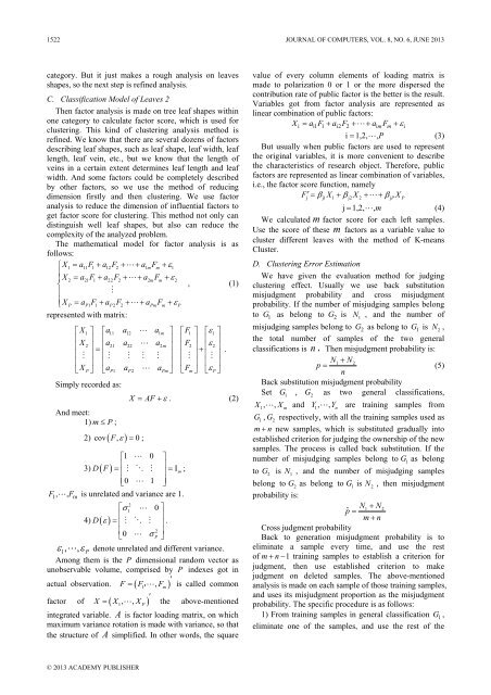
The mathematical model for factor analysis is as
follows:
⎧X1 = a11F1 + a12F2 + + a1 mFm
+ ε1
⎪X2 = a21F1+ a22F2 + + a2 mFm
+ ε
2
⎨
, (1)
⎪
⎪
⎩XP = aP 1F1 + aP2F2
+ + aPmFm + ε
P
represented with matrix:
⎡X1 ⎤ ⎡a11 a12 a1 m ⎤ ⎡F1
⎤ ⎡ε1
⎤
⎢
X
⎥ ⎢ ⎥
2
a21 a22 a
⎢
2m
F
⎥ ⎢
2
ε
⎥
⎢ ⎥ ⎢
2
= ⎥ ⎢ ⎥+
⎢ ⎥ .
⎢ ⎥ ⎢ ⎥ ⎢ ⎥ ⎢
⎥
⎢ ⎥ ⎢ ⎥ ⎢ ⎥ ⎢ ⎥
⎣X P⎦ ⎣aP1 aP2
aPm⎦
⎣Fm
⎦ ⎣ε
P⎦
Simply recorded as:
And meet:
1) m≤ P;
2) cov ( F, ε ) = 0 ;
X = AF + ε . (2)
⎡1 0 ⎤
3) D( F)
=
⎢ ⎥
⎢
⎥
= Im
;
⎢⎣0 1 ⎥⎦
F , , F is unrelated and variance are 1.
1 m
2
⎡σ
1
0 ⎤
⎢ ⎥
4) D ( ε ) = ⎢ ⎥ .
⎢
2
0 σ ⎥
⎣
P ⎦
ε
1,
,ε P
denote unrelated and different variance.
Among them is the P dimensional random vector as
unobservable volume, comprised by P indexes got in
F = F , F ′ is called common
actual observation. ( )
factor of ( )
1
,
m
X = X , , 1
X ′
P
the above-mentioned
integrated variable. A is factor loading matrix, on which
maximum variance rotation is made with variance, so that
the structure of A simplified. In other words, the square
value of every column elements of loading matrix is
made to polarization 0 or 1 or the more dispersed the
contribution rate of public factor is the better is the result.
Variables got from factor analysis are represented as
linear combination of public factors:
Xi = ai1F1+ ai2F2 + + aimFm
+ εi
i = 1,2, ,P
(3)
But usually when public factors are used to represent
the original variables, it is more convenient to describe
the characteristics of research object. Therefore, public
factors are represented as linear combination of variables,
i.e., the factor score function, namely
F′= β X + β X + + β X
j j1 1 j2 2 jP P
j= 1,2, ,m
(4)
We calculated m factor score for each left samples.
Use the score of these m factors as a variable value to
cluster different leaves with the method of K-means
Cluster.
D. Clustering Error Estimation
We have given the evaluation method for judging
clustering effect. Usually we use back substitution
misjudgment probability and cross misjudgment
probability. If the number of misjudging samples belong
to G 1 as belong to G2
is N
1
, and the number of
misjudging samples belong to G 2 as belong to G 1 is N
2
,
the total number of samples of the two general
classifications is n ,Then misjudgment probability is:
N1+
N2
p = (5)
n
Back substitution misjudgment probability
Set G
1
, G
2
as two general classifications,
X , , 1
X
m
and Y , , 1
Yn
are training samples from
G
1
, G
2
respectively, with all the training samples used as
m+ n new samples, which is substituted gradually into
established criterion for judging the ownership of the new
samples. The process is called back substitution. If the
number of misjudging samples belong to G 1
as belong
to G
2
is N
1
, and the number of misjudging samples
belong to G 2
as belong to G 1
is N
2
, then misjudgment
probability is:
N1+
N2
pˆ
=
m+
n
Cross judgment probability
Back to generation misjudgment probability is to
eliminate a sample every time, and use the rest
of m+ n− 1 training samples to establish a criterion for
judgment, then use established criterion to make
judgment on deleted samples. The above-mentioned
analysis is made on each sample of those training samples,
and uses its misjudgment proportion as the misjudgment
probability. The specific procedure is as follows:
1) From training samples in general classification G 1 ,
eliminate one of the samples, and use the rest of the
© 2013 ACADEMY PUBLISHER