- Page 3:
Structural Concrete
- Page 6 and 7:
Portions of this publication reprod
- Page 8 and 9:
vi Contents 2.9 Shear Modulus 24 2.
- Page 10 and 11:
viii Contents 8 Design of Deep Beam
- Page 12 and 13:
x Contents 14.9 Design Requirements
- Page 14 and 15:
xii Contents 21.5 Circular Beam Sub
- Page 16 and 17:
xiv Preface 5. To explain the failu
- Page 18 and 19:
xvi Preface A companion Web site fo
- Page 20 and 21:
xviii Notation C c C m C r C s C t
- Page 22 and 23:
xx Notation M 1s Factored end momen
- Page 24 and 25:
xxii Notation ζ Parameter for eval
- Page 26 and 27:
xxiv Conversion Factors To Convert
- Page 29 and 30:
CHAPTER1 INTRODUCTION Water Tower P
- Page 31 and 32:
1.3 Advantages and Disadvantages of
- Page 33 and 34:
1.6 Units of Measurement 5 A second
- Page 35 and 36:
1.7 Loads 7 Table 1.2 Density and S
- Page 37 and 38:
1.10 Structural Concrete Design 9 F
- Page 39 and 40:
1.12 Concrete High-Rise Buildings 1
- Page 41 and 42:
References 13 Concrete bridge, Knox
- Page 43 and 44:
CHAPTER2 PROPERTIES OF REINFORCED C
- Page 45 and 46:
2.2 Compressive Strength 17 Table 2
- Page 47 and 48:
2.4 Tensile Strength of Concrete 19
- Page 49 and 50:
2.6 Shear Strength 21 The splitting
- Page 51 and 52:
2.8 Poisson’s Ratio 23 For practi
- Page 53 and 54:
2.12 Creep 25 3. Type, Amount, and
- Page 55 and 56:
2.13 Models for Predicting Shrinkag
- Page 57 and 58:
2.13 Models for Predicting Shrinkag
- Page 59 and 60:
2.13 Models for Predicting Shrinkag
- Page 61 and 62:
2.13 Models for Predicting Shrinkag
- Page 63 and 64:
2.13 Models for Predicting Shrinkag
- Page 65 and 66:
2.13 Models for Predicting Shrinkag
- Page 67 and 68:
2.13 Models for Predicting Shrinkag
- Page 69 and 70:
2.13 Models for Predicting Shrinkag
- Page 71 and 72:
2.13 Models for Predicting Shrinkag
- Page 73 and 74:
2.13 Models for Predicting Shrinkag
- Page 75 and 76:
2.13 Models for Predicting Shrinkag
- Page 77 and 78:
2.13 Models for Predicting Shrinkag
- Page 79 and 80:
2.13 Models for Predicting Shrinkag
- Page 81 and 82:
2.13 Models for Predicting Shrinkag
- Page 83 and 84:
2.13 Models for Predicting Shrinkag
- Page 85 and 86:
2.13 Models for Predicting Shrinkag
- Page 87 and 88:
2.13 Models for Predicting Shrinkag
- Page 89 and 90:
2.13 Models for Predicting Shrinkag
- Page 91 and 92:
2.13 Models for Predicting Shrinkag
- Page 93 and 94:
2.13 Models for Predicting Shrinkag
- Page 95 and 96:
2.13 Models for Predicting Shrinkag
- Page 97 and 98:
2.14 Unit Weight of Concrete 69 Det
- Page 99 and 100:
2.17 Lightweight Concrete 71 Castin
- Page 101 and 102:
2.19 Steel Reinforcement 73 have pr
- Page 103 and 104:
2.19 Steel Reinforcement 75 Table 2
- Page 105 and 106:
2.19 Steel Reinforcement 77 Table 2
- Page 107 and 108:
References 79 Section 2.14 The unit
- Page 109 and 110:
Problems 81 2.10 Determine the modu
- Page 111 and 112:
CHAPTER3 FLEXURAL ANALYSIS OF REINF
- Page 113 and 114:
3.3 Behavior of Simply Supported Re
- Page 115 and 116:
3.3 Behavior of Simply Supported Re
- Page 117 and 118:
3.4 Types of Flexural Failure and S
- Page 119 and 120:
3.5 Load Factors 91 h c b d d t A s
- Page 121 and 122:
3.6 Strength Reduction Factor φ 93
- Page 123 and 124:
3.8 Equivalent Compressive Stress D
- Page 125 and 126:
3.8 Equivalent Compressive Stress D
- Page 127 and 128:
3.9 Singly Reinforced Rectangular S
- Page 129 and 130:
3.9 Singly Reinforced Rectangular S
- Page 131 and 132:
3.9 Singly Reinforced Rectangular S
- Page 133 and 134:
3.9 Singly Reinforced Rectangular S
- Page 135 and 136:
3.9 Singly Reinforced Rectangular S
- Page 137 and 138:
3.11 Adequacy of Sections 109 accom
- Page 139 and 140:
3.11 Adequacy of Sections 111 2. Ch
- Page 141 and 142:
3.12 Bundled Bars 113 2. Check ρ m
- Page 143 and 144:
3.13 Sections in the Transition Reg
- Page 145 and 146:
3.14 Rectangular Sections with Comp
- Page 147 and 148:
3.14 Rectangular Sections with Comp
- Page 149 and 150:
3.14 Rectangular Sections with Comp
- Page 151 and 152:
3.14 Rectangular Sections with Comp
- Page 153 and 154:
3.14 Rectangular Sections with Comp
- Page 155 and 156:
3.15 Analysis of T- and I-Sections
- Page 157 and 158:
3.15 Analysis of T- and I-Sections
- Page 159 and 160:
3.15 Analysis of T- and I-Sections
- Page 161 and 162:
3.15 Analysis of T- and I-Sections
- Page 163 and 164:
3.15 Analysis of T- and I-Sections
- Page 165 and 166:
3.18 Sections of Other Shapes 137 3
- Page 167 and 168:
3.19 Analysis of Sections Using Tab
- Page 169 and 170:
3.20 Additional Examples 141 Soluti
- Page 171 and 172:
3.21 Examples Using SI Units 143 Fo
- Page 173 and 174:
Summary 145 SUMMARY Flowcharts for
- Page 175 and 176:
Summary 147 Note that (A s f y −
- Page 177 and 178:
Problems 149 3.2 Rectangular sectio
- Page 179 and 180:
Problems 151 Figure 3.41 Problem 3.
- Page 181 and 182:
4.2 Rectangular Sections with Tensi
- Page 183 and 184:
4.3 Spacing of Reinforcement and Co
- Page 185 and 186:
4.3 Spacing of Reinforcement and Co
- Page 187 and 188:
4.3 Spacing of Reinforcement and Co
- Page 189 and 190:
4.3 Spacing of Reinforcement and Co
- Page 191 and 192:
4.4 Rectangular Sections with Compr
- Page 193 and 194:
4.4 Rectangular Sections with Compr
- Page 195 and 196:
4.4 Rectangular Sections with Compr
- Page 197 and 198:
4.5 Design of T-Sections 169 3. Com
- Page 199 and 200:
4.5 Design of T-Sections 171 The de
- Page 201 and 202:
4.5 Design of T-Sections 173 A s Fi
- Page 203 and 204:
4.6 Additional Examples 175 Example
- Page 205 and 206:
4.6 Additional Examples 177 1.5 2.3
- Page 207 and 208:
4.7 Examples Using SI Units 179 Sol
- Page 209 and 210:
Summary 181 SUMMARY Sections 4.1-4.
- Page 211 and 212:
Summary 183 There are two cases: Ca
- Page 213 and 214:
Problems 185 No. M u (K⋅ft) b (in
- Page 215 and 216:
Problems 187 Figure 4.17 Problem 4.
- Page 217 and 218:
5.2 Shear Stresses in Concrete Beam
- Page 219 and 220:
5.3 Behavior of Beams without Shear
- Page 221 and 222:
5.4 Moment Effect on Shear Strength
- Page 223 and 224:
5.5 Beams with Shear Reinforcement
- Page 225 and 226:
5.5 Beams with Shear Reinforcement
- Page 227 and 228:
5.6 ACI Code Shear Design Requireme
- Page 229 and 230:
5.7 Design of Vertical Stirrups 201
- Page 231 and 232:
5.7 Design of Vertical Stirrups 203
- Page 233 and 234:
5.8 Design Summary 205 5.8 DESIGN S
- Page 235 and 236:
5.8 Design Summary 207 Choose no. 3
- Page 237 and 238:
5.9 Shear Force Due to Live Loads 2
- Page 239 and 240:
5.9 Shear Force Due to Live Loads 2
- Page 241 and 242:
5.10 Shear Stresses in Members of V
- Page 243 and 244:
5.10 Shear Stresses in Members of V
- Page 245 and 246:
5.11 Examples Using SI Units 217 M
- Page 247 and 248:
5.11 Examples Using SI Units 219 Ta
- Page 249 and 250:
5.11 Examples Using SI Units 221 5.
- Page 251 and 252:
Problems 223 3. R. C. Fenwick and T
- Page 253 and 254:
Problems 225 11.1 K/ft Figure 5.25
- Page 255 and 256:
6.2 Instantaneous Deflection 227 Ta
- Page 257 and 258:
6.2 Instantaneous Deflection 229 wh
- Page 259 and 260:
6.2 Instantaneous Deflection 231 (a
- Page 261 and 262:
6.3 Long-Time Deflection 233 Then c
- Page 263 and 264:
6.5 Deflection Due to Combinations
- Page 265 and 266:
6.5 Deflection Due to Combinations
- Page 267 and 268:
6.5 Deflection Due to Combinations
- Page 269 and 270:
6.5 Deflection Due to Combinations
- Page 271 and 272:
6.6 Cracks in Flexural Members 243
- Page 273 and 274:
6.6 Cracks in Flexural Members 245
- Page 275 and 276:
6.7 ACI Code Requirements 247 have
- Page 277 and 278:
6.7 ACI Code Requirements 249 Check
- Page 279 and 280:
6.7 ACI Code Requirements 251 Choos
- Page 281 and 282:
References 253 2. Maximum crack wid
- Page 283 and 284:
Problems 255 Figure 6.13 Problem 6.
- Page 285 and 286:
CHAPTER7 DEVELOPMENT LENGTH OF REIN
- Page 287 and 288:
7.2 Development of Bond Stresses 25
- Page 289 and 290:
7.3 Development Length in Tension 2
- Page 291 and 292:
7.3 Development Length in Tension 2
- Page 293 and 294:
7.4 Development Length in Compressi
- Page 295 and 296:
7.5 Summary for Computation of I d
- Page 297 and 298:
7.6 Critical Sections in Flexural M
- Page 299 and 300:
7.6 Critical Sections in Flexural M
- Page 301 and 302:
7.7 Standard Hooks (ACI Code, Secti
- Page 303 and 304:
7.7 Standard Hooks (ACI Code, Secti
- Page 305 and 306:
7.8 Splices of Reinforcement 277 Fi
- Page 307 and 308:
7.8 Splices of Reinforcement 279 So
- Page 309 and 310:
7.9 Moment-Resistance Diagram (Bar
- Page 311 and 312:
7.9 Moment-Resistance Diagram (Bar
- Page 313 and 314:
Summary 285 Let A s = 0.018(10)(17)
- Page 315 and 316:
Problems 287 7. C. O. Orangum, J. O
- Page 317 and 318:
Problems 289 Figure 7.17 (33 kN/m).
- Page 319 and 320:
8.3 Strut-and-Tie Model 291 D B D D
- Page 321 and 322:
8.4 ACI Design Procedure to Build a
- Page 323 and 324:
8.4 ACI Design Procedure to Build a
- Page 325 and 326:
8.4 ACI Design Procedure to Build a
- Page 327 and 328:
8.4 ACI Design Procedure to Build a
- Page 329 and 330:
8.5 Strut-and-Tie Method According
- Page 331 and 332:
8.6 Deep Members 303 This equation
- Page 333 and 334:
8.6 Deep Members 305 that cause cra
- Page 335 and 336:
8.6 Deep Members 307 P u = 768 K D
- Page 337 and 338:
8.6 Deep Members 309 Strut Nodal zo
- Page 339 and 340:
8.6 Deep Members 311 V u = 160 K CL
- Page 341 and 342:
8.6 Deep Members 313 Centroid of st
- Page 343 and 344:
8.6 Deep Members 315 2. Check if be
- Page 345 and 346:
8.6 Deep Members 317 9. Check ancho
- Page 347 and 348:
8.6 Deep Members 319 Pu = 766 K 6.0
- Page 349 and 350:
References 321 No. 9 bar @3.5" c/c
- Page 351 and 352:
Problems 323 11.3’ 11.3’ W LL W
- Page 353 and 354: 9.1 Types of Slabs 325 (a) (b) (c)
- Page 355 and 356: 9.2 Design of One-Way Solid Slabs 3
- Page 357 and 358: 9.6 Distribution of Loads from One-
- Page 359 and 360: 9.6 Distribution of Loads from One-
- Page 361 and 362: 9.6 Distribution of Loads from One-
- Page 363 and 364: 9.7 One-Way Joist Floor System 335
- Page 365 and 366: 9.7 One-Way Joist Floor System 337
- Page 367 and 368: References 339 One-way ribbed slab
- Page 369 and 370: Problems 341 9.6 Repeat Problem 9.4
- Page 371 and 372: 10.2 Types of Columns 343 Figure 10
- Page 373 and 374: 10.4 ACI Code Limitations 345 (a) (
- Page 375 and 376: 10.5 Spiral Reinforcement 347 Table
- Page 377 and 378: 10.8 Long Columns 349 reinforced co
- Page 379 and 380: 10.8 Long Columns 351 3. Design of
- Page 381 and 382: References 353 Section 10.5 Minimum
- Page 383 and 384: Problems 355 Number f ′ c (ksi) P
- Page 385 and 386: 11.1 Introduction 357 B C H A A D V
- Page 387 and 388: 11.3 Load-Moment Interaction Diagra
- Page 389 and 390: 11.4 Safety Provisions 361 11.4 SAF
- Page 391 and 392: 11.5 Balanced Condition: Rectangula
- Page 393 and 394: 11.6 Column Sections under Eccentri
- Page 395 and 396: 11.7 Strength of Columns for Tensio
- Page 397 and 398: 11.7 Strength of Columns for Tensio
- Page 399 and 400: 11.8 Strength of Columns for Compre
- Page 401 and 402: 11.8 Strength of Columns for Compre
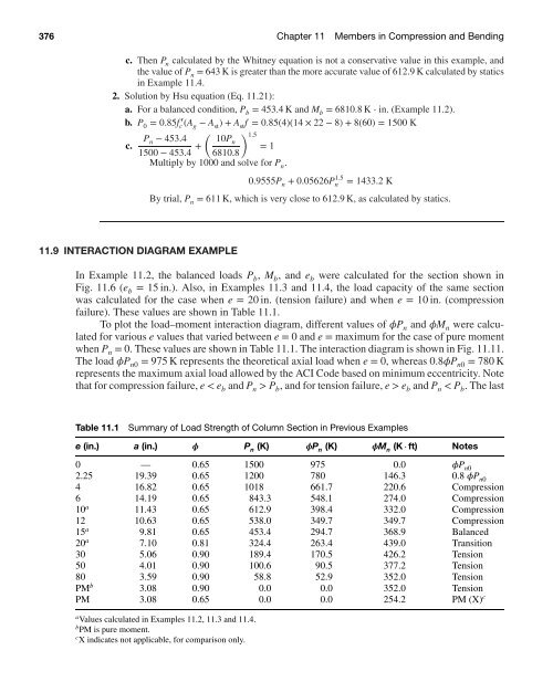
- Page 403: 11.8 Strength of Columns for Compre
- Page 407 and 408: 11.10 Rectangular Columns with Side
- Page 409 and 410: 11.11 Load Capacity of Circular Col
- Page 411 and 412: 11.11 Load Capacity of Circular Col
- Page 413 and 414: 11.11 Load Capacity of Circular Col
- Page 415 and 416: 11.12 Analysis and Design of Column
- Page 417 and 418: 11.12 Analysis and Design of Column
- Page 419 and 420: 11.13 Design of Columns under Eccen
- Page 421 and 422: 11.13 Design of Columns under Eccen
- Page 423 and 424: 11.13 Design of Columns under Eccen
- Page 425 and 426: 11.14 Biaxial Bending 397 5 no. 10
- Page 427 and 428: 11.15 Circular Columns with Uniform
- Page 429 and 430: 11.15 Circular Columns with Uniform
- Page 431 and 432: 11.17 Parme Load Contour Method 403
- Page 433 and 434: 11.17 Parme Load Contour Method 405
- Page 435 and 436: 11.17 Parme Load Contour Method 407
- Page 437 and 438: 11.18 Equation of Failure Surface 4
- Page 439 and 440: 11.19 SI Example 411 3. Compute the
- Page 441 and 442: Summary 413 SUMMARY Sections 11.1-1
- Page 443 and 444: Problems 415 REFERENCES 1. B. Brest
- Page 445 and 446: Problems 417 16 no. 10 bars Figure
- Page 447 and 448: Problems 419 11.12 Repeat Problem 1
- Page 449 and 450: 12.2 Effective Column Length (Kl u
- Page 451 and 452: 12.3 Effective Length Factor (K) 42
- Page 453 and 454: 12.4 Member Stiffness (EI) 425 Long
- Page 455 and 456:
12.5 Limitation of the Slenderness
- Page 457 and 458:
12.6 Moment-Magnifier Design Method
- Page 459 and 460:
12.6 Moment-Magnifier Design Method
- Page 461 and 462:
12.6 Moment-Magnifier Design Method
- Page 463 and 464:
12.6 Moment-Magnifier Design Method
- Page 465 and 466:
12.6 Moment-Magnifier Design Method
- Page 467 and 468:
Summary 439 3. The value of K can b
- Page 469 and 470:
Problems 441 7. R. Green and J. E.
- Page 471 and 472:
CHAPTER13 FOOTINGS Office building
- Page 473 and 474:
13.2 Types of Footings 445 Vertical
- Page 475 and 476:
13.2 Types of Footings 447 Figure 1
- Page 477 and 478:
13.4 Design Considerations 449 Figu
- Page 479 and 480:
13.4 Design Considerations 451 This
- Page 481 and 482:
13.4 Design Considerations 453 c Co
- Page 483 and 484:
13.4 Design Considerations 455 Figu
- Page 485 and 486:
13.4 Design Considerations 457 Figu
- Page 487 and 488:
13.5 Plain Concrete Footings 459 th
- Page 489 and 490:
13.5 Plain Concrete Footings 461 No
- Page 491 and 492:
13.5 Plain Concrete Footings 463 c
- Page 493 and 494:
13.5 Plain Concrete Footings 465 Th
- Page 495 and 496:
13.5 Plain Concrete Footings 467 8'
- Page 497 and 498:
13.5 Plain Concrete Footings 469 14
- Page 499 and 500:
13.5 Plain Concrete Footings 471 Fi
- Page 501 and 502:
13.6 Combined Footings 473 Figure 1
- Page 503 and 504:
13.6 Combined Footings 475 (Assumed
- Page 505 and 506:
13.6 Combined Footings 477 16″ ×
- Page 507 and 508:
13.8 Footings under Biaxial Moment
- Page 509 and 510:
13.8 Footings under Biaxial Moment
- Page 511 and 512:
13.10 Footings on Piles 483 13.9 SL
- Page 513 and 514:
Summary 485 V Required d = u (1000)
- Page 515 and 516:
Problems 487 Section 13.5 Plain con
- Page 517 and 518:
Problems 489 Table 13.3 Problem 13.
- Page 519 and 520:
14.2 Types of Retaining Walls 491 F
- Page 521 and 522:
14.4 Active and Passive Soil Pressu
- Page 523 and 524:
14.4 Active and Passive Soil Pressu
- Page 525 and 526:
14.5 Effect of Surcharge 497 The ac
- Page 527 and 528:
14.7 Stability Against Overturning
- Page 529 and 530:
14.9 Design Requirements 501 Figure
- Page 531 and 532:
14.10 Drainage 503 Example 14.1 The
- Page 533 and 534:
14.10 Drainage 505 c. The flexural
- Page 535 and 536:
14.10 Drainage 507 Figure 14.12 Exa
- Page 537 and 538:
14.10 Drainage 509 The total resist
- Page 539 and 540:
14.10 Drainage 511 concrete on the
- Page 541 and 542:
14.11 Basement Walls 513 Figure 14.
- Page 543 and 544:
14.11 Basement Walls 515 No. 4 @ 12
- Page 545 and 546:
Summary 517 Figure 14.17 Example 14
- Page 547 and 548:
Problems 519 Figure 14.18 Problem 1
- Page 549 and 550:
Problems 521 the coefficient of fri
- Page 551 and 552:
CHAPTER15 DESIGN FOR TORSION Apartm
- Page 553 and 554:
15.3 Torsional Stresses 525 Figure
- Page 555 and 556:
15.3 Torsional Stresses 527 Table 1
- Page 557 and 558:
15.6 Torsion Theories for Concrete
- Page 559 and 560:
15.6 Torsion Theories for Concrete
- Page 561 and 562:
15.6 Torsion Theories for Concrete
- Page 563 and 564:
15.8 Torsion in Reinforced Concrete
- Page 565 and 566:
15.8 Torsion in Reinforced Concrete
- Page 567 and 568:
15.8 Torsion in Reinforced Concrete
- Page 569 and 570:
15.8 Torsion in Reinforced Concrete
- Page 571 and 572:
15.9 Summary of ACI Code Procedures
- Page 573 and 574:
15.9 Summary of ACI Code Procedures
- Page 575 and 576:
15.9 Summary of ACI Code Procedures
- Page 577 and 578:
15.9 Summary of ACI Code Procedures
- Page 579 and 580:
References 551 Equation U.S. Custom
- Page 581 and 582:
Problems 553 3 no. 9 Figure 15.17 P
- Page 583 and 584:
CHAPTER16 CONTINUOUS BEAMS AND FRAM
- Page 585 and 586:
16.2 Maximum Moments in Continuous
- Page 587 and 588:
16.2 Maximum Moments in Continuous
- Page 589 and 590:
16.3 Building Frames 561 2 no. 9 4
- Page 591 and 592:
16.4 Portal Frames 563 Figure 16.8
- Page 593 and 594:
16.6 Design of Frame Hinges 565 For
- Page 595 and 596:
16.6 Design of Frame Hinges 567 Fig
- Page 597 and 598:
16.6 Design of Frame Hinges 569 Fig
- Page 599 and 600:
16.6 Design of Frame Hinges 571 Fig
- Page 601 and 602:
16.6 Design of Frame Hinges 573 d.
- Page 603 and 604:
16.6 Design of Frame Hinges 575 Fro
- Page 605 and 606:
16.6 Design of Frame Hinges 577 iii
- Page 607 and 608:
16.7 Introduction to Limit Design 5
- Page 609 and 610:
16.8 The Collapse Mechanism 581 tra
- Page 611 and 612:
16.11 Limit Analysis 583 Example 16
- Page 613 and 614:
16.11 Limit Analysis 585 Figure 16.
- Page 615 and 616:
16.12 Rotation of Plastic Hinges 58
- Page 617 and 618:
16.12 Rotation of Plastic Hinges 58
- Page 619 and 620:
16.12 Rotation of Plastic Hinges 59
- Page 621 and 622:
16.13 Summary of Limit Design Proce
- Page 623 and 624:
16.13 Summary of Limit Design Proce
- Page 625 and 626:
16.14 Moment Redistribution of Maxi
- Page 627 and 628:
16.14 Moment Redistribution of Maxi
- Page 629 and 630:
16.14 Moment Redistribution of Maxi
- Page 631 and 632:
16.14 Moment Redistribution of Maxi
- Page 633 and 634:
Summary 605 A B C D E F Typical sec
- Page 635 and 636:
Problems 607 Table 16.1 gives the d
- Page 637 and 638:
Problems 609 Figure 16.36 Problem 1
- Page 639 and 640:
17.2 Types of Two-Way Slabs 611 Fig
- Page 641 and 642:
17.2 Types of Two-Way Slabs 613 Fig
- Page 643 and 644:
17.4 Design Concepts 615 Slabonbeam
- Page 645 and 646:
17.4 Design Concepts 617 Figure 17.
- Page 647 and 648:
17.5 Column and Middle Strips 619 T
- Page 649 and 650:
17.6 Minimum Slab Thickness to Cont
- Page 651 and 652:
17.6 Minimum Slab Thickness to Cont
- Page 653 and 654:
17.7 Shear Strength of Slabs 625 Fi
- Page 655 and 656:
17.7 Shear Strength of Slabs 627 Fi
- Page 657 and 658:
17.8 Analysis of Two-Way Slabs by t
- Page 659 and 660:
17.8 Analysis of Two-Way Slabs by t
- Page 661 and 662:
17.8 Analysis of Two-Way Slabs by t
- Page 663 and 664:
17.8 Analysis of Two-Way Slabs by t
- Page 665 and 666:
17.8 Analysis of Two-Way Slabs by t
- Page 667 and 668:
17.8 Analysis of Two-Way Slabs by t
- Page 669 and 670:
17.8 Analysis of Two-Way Slabs by t
- Page 671 and 672:
17.8 Analysis of Two-Way Slabs by t
- Page 673 and 674:
17.8 Analysis of Two-Way Slabs by t
- Page 675 and 676:
17.8 Analysis of Two-Way Slabs by t
- Page 677 and 678:
17.8 Analysis of Two-Way Slabs by t
- Page 679 and 680:
17.8 Analysis of Two-Way Slabs by t
- Page 681 and 682:
17.8 Analysis of Two-Way Slabs by t
- Page 683 and 684:
17.8 Analysis of Two-Way Slabs by t
- Page 685 and 686:
17.8 Analysis of Two-Way Slabs by t
- Page 687 and 688:
17.10 Transfer of Unbalanced Moment
- Page 689 and 690:
17.10 Transfer of Unbalanced Moment
- Page 691 and 692:
17.10 Transfer of Unbalanced Moment
- Page 693 and 694:
17.10 Transfer of Unbalanced Moment
- Page 695 and 696:
17.10 Transfer of Unbalanced Moment
- Page 697 and 698:
17.10 Transfer of Unbalanced Moment
- Page 699 and 700:
17.10 Transfer of Unbalanced Moment
- Page 701 and 702:
(a) Figure 17.33 (a) Planofthewaffl
- Page 703 and 704:
17.11 Waffle Slabs 675 Table 17.12
- Page 705 and 706:
17.11 Waffle Slabs 677 (a) (b) M 0
- Page 707 and 708:
17.11 Waffle Slabs 679 Table 17.13
- Page 709 and 710:
17.12 Equivalent Frame Method 681 b
- Page 711 and 712:
17.12 Equivalent Frame Method 683 t
- Page 713 and 714:
17.12 Equivalent Frame Method 685 T
- Page 715 and 716:
17.12 Equivalent Frame Method 687 F
- Page 717 and 718:
17.12 Equivalent Frame Method 689 F
- Page 719 and 720:
17.12 Equivalent Frame Method 691 T
- Page 721 and 722:
Problems 693 Section 17.12 1. In th
- Page 723 and 724:
Problems 695 17.5 (Flat slabs) Use
- Page 725 and 726:
18.1 Introduction 697 Figure 18.1 P
- Page 727 and 728:
18.2 Types of Stairs 699 Figure 18.
- Page 729 and 730:
18.2 Types of Stairs 701 Figure 18.
- Page 731 and 732:
18.2 Types of Stairs 703 Figure 18.
- Page 733 and 734:
18.2 Types of Stairs 705 Figure 18.
- Page 735 and 736:
18.2 Types of Stairs 707 Free-stand
- Page 737 and 738:
18.2 Types of Stairs 709 Figure 18.
- Page 739 and 740:
18.2 Types of Stairs 711 For a symm
- Page 741 and 742:
18.3 Examples 713 2. The width of s
- Page 743 and 744:
18.3 Examples 715 Let d = 7.9 − 0
- Page 745 and 746:
18.3 Examples 717 1 no. 3 / step No
- Page 747 and 748:
18.3 Examples 719 6. The transverse
- Page 749 and 750:
Summary 721 3. Calculate the reinfo
- Page 751 and 752:
Problems 723 Figure 18.23 Problem 1
- Page 753 and 754:
19.1 Prestressed Concrete 725 Figur
- Page 755 and 756:
19.1 Prestressed Concrete 727 f ′
- Page 757 and 758:
19.1 Prestressed Concrete 729 Addin
- Page 759 and 760:
19.1 Prestressed Concrete 731 may b
- Page 761 and 762:
19.1 Prestressed Concrete 733 Figur
- Page 763 and 764:
19.2 Materials and Serviceability R
- Page 765 and 766:
19.3 Loss of Prestress 737 Table 19
- Page 767 and 768:
19.3 Loss of Prestress 739 and ( Fi
- Page 769 and 770:
19.3 Loss of Prestress 741 where P
- Page 771 and 772:
19.3 Loss of Prestress 743 2. Loss
- Page 773 and 774:
19.3 Loss of Prestress 745 4. Loss
- Page 775 and 776:
19.4 Analysis of Flexural Members 7
- Page 777 and 778:
19.4 Analysis of Flexural Members 7
- Page 779 and 780:
19.4 Analysis of Flexural Members 7
- Page 781 and 782:
19.4 Analysis of Flexural Members 7
- Page 783 and 784:
19.4 Analysis of Flexural Members 7
- Page 785 and 786:
19.5 Design of Flexural Members 757
- Page 787 and 788:
19.5 Design of Flexural Members 759
- Page 789 and 790:
19.5 Design of Flexural Members 761
- Page 791 and 792:
19.6 Cracking Moment 763 The maximu
- Page 793 and 794:
19.7 Deflection 765 called camber.
- Page 795 and 796:
19.8 Design for Shear 767 The cambe
- Page 797 and 798:
19.8 Design for Shear 769 Figure 19
- Page 799 and 800:
19.8 Design for Shear 771 3. The mi
- Page 801 and 802:
19.8 Design for Shear 773 Use d p =
- Page 803 and 804:
19.9 Preliminary Design of Prestres
- Page 805 and 806:
19.10 End-Block Stresses 777 The co
- Page 807 and 808:
19.10 End-Block Stresses 779 Figure
- Page 809 and 810:
Summary 781 Section 19.5 The nomina
- Page 811 and 812:
Problems 783 27. Y. Guyon. Prestres
- Page 813 and 814:
Problems 785 b. Locate the tendons
- Page 815 and 816:
20.2 Seismic Design Category 787 20
- Page 817 and 818:
20.2 Seismic Design Category 789 Ta
- Page 819 and 820:
20.2 Seismic Design Category 791 Fi
- Page 821 and 822:
20.2 Seismic Design Category 793 Fi
- Page 823 and 824:
20.2 Seismic Design Category 795 Ta
- Page 825 and 826:
20.2 Seismic Design Category 797 Fi
- Page 827 and 828:
20.2 Seismic Design Category 799 Fi
- Page 829 and 830:
20.2 Seismic Design Category 801 Fi
- Page 831 and 832:
20.2 Seismic Design Category 803 St
- Page 833 and 834:
20.3 Analysis Procedures 805 Table
- Page 835 and 836:
20.3 Analysis Procedures 807 The la
- Page 837 and 838:
20.3 Analysis Procedures 809 Step 5
- Page 839 and 840:
20.3 Analysis Procedures 811 Table
- Page 841 and 842:
20.3 Analysis Procedures 813 Exampl
- Page 843 and 844:
20.3 Analysis Procedures 815 254 6
- Page 845 and 846:
20.3 Analysis Procedures 817 9. Det
- Page 847 and 848:
20.5 Special Requirements in Design
- Page 849 and 850:
20.5 Special Requirements in Design
- Page 851 and 852:
20.5 Special Requirements in Design
- Page 853 and 854:
20.5 Special Requirements in Design
- Page 855 and 856:
20.5 Special Requirements in Design
- Page 857 and 858:
20.5 Special Requirements in Design
- Page 859 and 860:
20.5 Special Requirements in Design
- Page 861 and 862:
20.5 Special Requirements in Design
- Page 863 and 864:
20.5 Special Requirements in Design
- Page 865 and 866:
20.5 Special Requirements in Design
- Page 867 and 868:
20.5 Special Requirements in Design
- Page 869 and 870:
20.5 Special Requirements in Design
- Page 871 and 872:
20.5 Special Requirements in Design
- Page 873 and 874:
20.5 Special Requirements in Design
- Page 875 and 876:
20.5 Special Requirements in Design
- Page 877 and 878:
20.5 Special Requirements in Design
- Page 879 and 880:
20.5 Special Requirements in Design
- Page 881 and 882:
20.5 Special Requirements in Design
- Page 883 and 884:
20.5 Special Requirements in Design
- Page 885 and 886:
Problems 857 20.5 Design the transv
- Page 887 and 888:
21.2 Uniformly Loaded Circular Beam
- Page 889 and 890:
21.2 Uniformly Loaded Circular Beam
- Page 891 and 892:
21.2 Uniformly Loaded Circular Beam
- Page 893 and 894:
21.3 Semicircular Beam Fixed at End
- Page 895 and 896:
21.3 Semicircular Beam Fixed at End
- Page 897 and 898:
21.4 Fixed-End Semicircular Beam un
- Page 899 and 900:
21.4 Fixed-End Semicircular Beam un
- Page 901 and 902:
21.5 Circular Beam Subjected to Uni
- Page 903 and 904:
21.6 Circular Beam Subjected to a C
- Page 905 and 906:
21.6 Circular Beam Subjected to a C
- Page 907 and 908:
21.7 V-Shape Beams Subjected to Uni
- Page 909 and 910:
21.8 V-Shape Beams Subjected to a C
- Page 911 and 912:
21.8 V-Shape Beams Subjected to a C
- Page 913 and 914:
Summary 885 Figure 21.12 Example 21
- Page 915 and 916:
CHAPTER22 PRESTRESSED CONCRETE BRID
- Page 917 and 918:
22.2 Typical Cross Sections 889 22.
- Page 919 and 920:
22.3 Design Philosophy of AASHTO Sp
- Page 921 and 922:
22.4 Load Factors and Combinations
- Page 923 and 924:
22.4 Load Factors and Combinations
- Page 925 and 926:
22.5 Gravity Loads 897 Table 22.10
- Page 927 and 928:
22.5 Gravity Loads 899 Design tande
- Page 929 and 930:
22.5 Gravity Loads 901 Table 22.12
- Page 931 and 932:
22.5 Gravity Loads 903 Table 22.13
- Page 933 and 934:
22.6 Design for Flexural and Axial
- Page 935 and 936:
22.7 Design for Shear (AASHTO 5.8)
- Page 937 and 938:
22.7 Design for Shear (AASHTO 5.8)
- Page 939 and 940:
22.7 Design for Shear (AASHTO 5.8)
- Page 941 and 942:
22.8 Loss of Prestress (AASHTO 5.9.
- Page 943 and 944:
22.9 Deflections (AASHTO 5.7.3.6) 9
- Page 945 and 946:
22.9 Deflections (AASHTO 5.7.3.6) 9
- Page 947 and 948:
22.9 Deflections (AASHTO 5.7.3.6) 9
- Page 949 and 950:
22.9 Deflections (AASHTO 5.7.3.6) 9
- Page 951 and 952:
22.9 Deflections (AASHTO 5.7.3.6) 9
- Page 953 and 954:
22.9 Deflections (AASHTO 5.7.3.6) 9
- Page 955 and 956:
22.9 Deflections (AASHTO 5.7.3.6) 9
- Page 957 and 958:
22.9 Deflections (AASHTO 5.7.3.6) 9
- Page 959 and 960:
22.9 Deflections (AASHTO 5.7.3.6) 9
- Page 961 and 962:
22.9 Deflections (AASHTO 5.7.3.6) 9
- Page 963 and 964:
22.9 Deflections (AASHTO 5.7.3.6) 9
- Page 965 and 966:
22.9 Deflections (AASHTO 5.7.3.6) 9
- Page 967 and 968:
22.9 Deflections (AASHTO 5.7.3.6) 9
- Page 969 and 970:
22.9 Deflections (AASHTO 5.7.3.6) 9
- Page 971 and 972:
22.9 Deflections (AASHTO 5.7.3.6) 9
- Page 973 and 974:
CHAPTER23 REVIEW PROBLEMS ON CONCRE
- Page 975 and 976:
Review Problems on Concrete Buildin
- Page 977 and 978:
Review Problems on Concrete Buildin
- Page 979 and 980:
Review Problems on Concrete Buildin
- Page 981 and 982:
Review Problems on Concrete Buildin
- Page 983 and 984:
Review Problems on Concrete Buildin
- Page 985 and 986:
Review Problems on Concrete Buildin
- Page 987 and 988:
Review Problems on Concrete Buildin
- Page 989 and 990:
Review Problems on Concrete Buildin
- Page 991 and 992:
Review Problems on Concrete Buildin
- Page 993 and 994:
Review Problems on Concrete Buildin
- Page 995 and 996:
Review Problems on Concrete Buildin
- Page 997 and 998:
Review Problems on Concrete Buildin
- Page 999 and 1000:
Design and Analysis Flowcharts 971
- Page 1001 and 1002:
Design and Analysis Flowcharts 973
- Page 1003 and 1004:
Design and Analysis Flowcharts 975
- Page 1005 and 1006:
Design and Analysis Flowcharts 977
- Page 1007 and 1008:
Design and Analysis Flowcharts 979
- Page 1009 and 1010:
Design and Analysis Flowcharts 981
- Page 1011 and 1012:
Design and Analysis Flowcharts 983
- Page 1013 and 1014:
Design and Analysis Flowcharts 985
- Page 1015 and 1016:
Design and Analysis Flowcharts 987
- Page 1017 and 1018:
Design and Analysis Flowcharts 989
- Page 1019 and 1020:
Design and Analysis Flowcharts 991
- Page 1021 and 1022:
Design and Analysis Flowcharts 993
- Page 1023 and 1024:
Appendix A Design Tables (U.S. Cust
- Page 1025 and 1026:
Appendix A Design Tables (U.S. Cust
- Page 1027 and 1028:
Appendix A Design Tables (U.S. Cust
- Page 1029 and 1030:
Appendix A Design Tables (U.S. Cust
- Page 1031:
Appendix A Design Tables (U.S. Cust
- Page 1034 and 1035:
1006 Appendix B Design Tables (SI U
- Page 1036 and 1037:
1008 Appendix B Design Tables (SI U
- Page 1038 and 1039:
1010 Appendix B Design Tables (SI U
- Page 1040 and 1041:
1012 Appendix B Design Tables (SI U
- Page 1042 and 1043:
1014 Appendix C Structural Aids Tab
- Page 1044 and 1045:
1016 Appendix C Structural Aids Tab
- Page 1046 and 1047:
1018 Appendix C Structural Aids Tab
- Page 1048 and 1049:
1020 Appendix C Structural Aids Tab
- Page 1050 and 1051:
1022 Appendix C Structural Aids Tab
- Page 1052 and 1053:
1024 Appendix C Structural Aids Tab
- Page 1054 and 1055:
1026 Appendix C Structural Aids Tab
- Page 1056 and 1057:
1028 Appendix C Structural Aids Tab
- Page 1058 and 1059:
1030 Appendix C Structural Aids Tab
- Page 1060 and 1061:
1032 Appendix C Structural Aids Tab
- Page 1062 and 1063:
1034 Index Beams (continued) stress
- Page 1064 and 1065:
1036 Index F Factored loads, 91 Fai
- Page 1066 and 1067:
1038 Index Seismic design (continue