STX Signal Transmitter Installation and Operation ... - Kistler-Morse

Chapter 3. Stand-Alone STX Analog Calibration and Setup
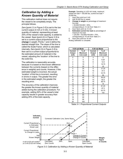
Calibration by Adding a
Known Quantity of Material
This calibration method does not require
the vessel to be completely empty. The
principle follows.
Zero [point (1) in Figure 3-3] is set to the low
current output (4 mA or 0 mA). A known
quantity of material, representing at least
25% of the vessel’s total capacity, is added to
the vessel. Span [point (2) in Figure 3-3] is
set to a current output proportional to the
change in weight. Points 1 and 2 define the
dashed straight line. The slope of the line is
called the Scale Factor, which is calculated
internally. Zero [point (3) in Figure 3-3] is
then set to a current output proportional to
the estimated amount of material in the
vessel, adjusting the ‘location’ of the line to
the solid line.
The calibration is reasonably accurate,
because it is based on the known difference
between the currents (based on the difference
in weights) and counts. However, if the
estimated weight is incorrect, the actual
‘location’ of the line is incorrect, resulting
in errors in output. The greater the error
in the estimated weight, the greater the
resulting error.
The accuracy of the calibration improves
the greater the known quantity of material
added during the calibration procedure. For
example, adding 50% of the vessel’s total
capacity results in greater accuracy than
adding 25% of the total capacity.
Example: Operating in 4-20 mA mode, maximum
vessel live load = 100,000 lbs, current live load =
25,000 lbs.
1. Input Zero point as 4 mA.
2. Add 50,000 lbs to vessel.
3. Change in weight as percentage of maximum
live load
= 50,000/100,000 = 50%,
corresponding to 12 mA from Table 3-1.
4. Input Span point as 12 mA.
5. Estimated current live load as percentage of
maximum live load
= (25,000 + 50,000)/100,000 = 75%,
corresponding to 16 mA from Table 3-1.
6. Input Zero point as 16 mA.
Analog calibration is complete.
0-20 mA Mode 4-20 mA Mode
Current % of Current % of
Output Maximum Output Maximum
(mA) Live Load (mA) Live Load
0 0 4 0
1 5 5 6.25
2 10 6 12.5
3 15 7 18.75
4 20 8 25
5 25 9 31.25
6 30 10 37.5
7 35 11 43.75
8 40 12 50
9 45 13 56.25
10 50 14 62.5
11 55 15 68.75
12 60 16 75
13 65 17 81.25
14 70 18 87.5
15 75 19 93.75
16 80 20 100
17 85
18 90
19 95
20 100
Table 3-1. Proportional Current Outputs
Indicated
Current
Current Proportional
to Estimated
Actual Load
Corrected Calibration Line, Same Slope
Zero
(3)
Current Proportional
to Change in Load (2)
Add
Known Weight
4 mA (4-20 mA mode)
or 0 mA (0-20 mA mode)
Calculated
Zero Counts
(1)
Zero
Span
Slope =
Change in Current
Change in Counts
Calculated
Span Counts
Figure 3-3. Calibration by Adding a Known Quantity of Material
Weight
Signal
in Counts
3-3