Processus de Lévy en Finance - Laboratoire de Probabilités et ...

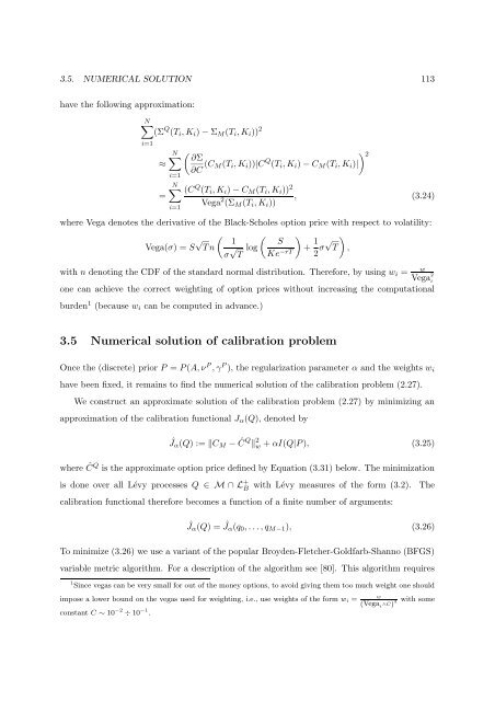
3.5. NUMERICAL SOLUTION 113
have the following approximation:
N∑
(Σ Q (T i , K i ) − Σ M (T i , K i )) 2
i=1
≈
=
N∑
i=1
( ) ∂Σ
2
∂C (C M(T i , K i ))|C Q (T i , K i ) − C M (T i , K i )|
N∑ (C Q (T i , K i ) − C M (T i , K i )) 2
Vega 2 , (3.24)
(Σ M (T i , K i ))
i=1
where Vega denotes the derivative of the Black-Scholes option price with respect to volatility:
Vega(σ) = S √ ( ( )
1 S
T n
σ √ T log Ke −rT + 1 )
2 σ√ T ,
with n denoting the CDF of the standard normal distribution. Therefore, by using w i =
w
Vega 2 i
one can achieve the correct weighting of option prices without increasing the computational
burden 1 (because w i can be computed in advance.)
3.5 Numerical solution of calibration problem
Once the (discrete) prior P = P (A, ν P , γ P ), the regularization parameter α and the weights w i
have been fixed, it remains to find the numerical solution of the calibration problem (2.27).
We construct an approximate solution of the calibration problem (2.27) by minimizing an
approximation of the calibration functional J α (Q), denoted by
Ĵ α (Q) := ‖C M − ĈQ ‖ 2 w + αI(Q|P ), (3.25)
where ĈQ is the approximate option price defined by Equation (3.31) below. The minimization
is done over all Lévy processes Q ∈ M ∩ L + B
with Lévy measures of the form (3.2). The
calibration functional therefore becomes a function of a finite number of arguments:
Ĵ α (Q) = Ĵα(q 0 , . . . , q M−1 ), (3.26)
To minimize (3.26) we use a variant of the popular Broyden-Fletcher-Goldfarb-Shanno (BFGS)
variable metric algorithm. For a description of the algorithm see [80]. This algorithm requires
1 Since vegas can be very small for out of the money options, to avoid giving them too much weight one should
impose a lower bound on the vegas used for weighting, i.e., use weights of the form w i =
constant C ∼ 10 −2 ÷ 10 −1 .
w
(Vega i ∧C) 2
with some