Processus de Lévy en Finance - Laboratoire de Probabilités et ...

5.2. SIMULATION OF DEPENDENT LEVY PROCESSES 181
8
1
7
0.5
6
0
5
−0.5
4
−1
3
−1.5
2
−2
1
−2.5
0
−3
−1
−3.5
−2
0 0.1 0.2 0.3 0.4 0.5 0.6 0.7 0.8 0.9 1
−4
0 0.1 0.2 0.3 0.4 0.5 0.6 0.7 0.8 0.9 1
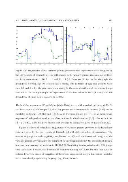
Figure 5.4: Trajectories of two variance gamma processes with dependence structure given by
the Lévy copula of Example 5.1. In both graphs both variance gamma processes are driftless
and have parameters c = 10, λ − = 1 and λ + = 1 (cf. Equation (1.19)). In the left graph, the
dependence between the two components is strong both in terms of sign and absolute value
(η = 0.9 and θ = 3): the processes jump mostly in the same direction and the sizes of jumps
are similar. In the right graph the dependence of absolute values is weak (θ = 0.5) and the
dependence of jump sign is negative (η = 0.25).
If ν is a Lévy measure on R 2 , satisfying ∫ (|x|∧1)ν(dx) < ∞ with marginal tail integrals U 1 , U 2
and Lévy copula F of Example 5.1, the Lévy process with characteristic function (5.13) can be
simulated as follows. Let {V i } and {Γ 1 i } be as in Theorem 5.6 and let {W i} be an independent
sequence of independent random variables, uniformly distributed on [0, 1].
For each i, let
Γ 2 i = F −1 (W
Γ 1 i ). Then the Lévy process that we want to simulate is given by Equation (5.12).
i
Figure 5.4 shows the simulated trajectories of variance gamma processes with dependence
structure given by the Lévy copula of Example 5.1 with different values of parameters. The
number of jumps for each trajectory was limited to 2000 and the inverse tail integral of the
variance gamma Lévy measure was computed by inverting numerically the exponential integral
function (function expint available in MATLAB). Simulating two trajectories with 2000 jumps
each takes about 1 second on a Pentium III computer running MATLAB, but this time could be
reduced by several orders of magnitude if the inverse exponential integral function is tabulated
and a lower-level programming language (e.g. C++) is used.