Processus de Lévy en Finance - Laboratoire de Probabilités et ...

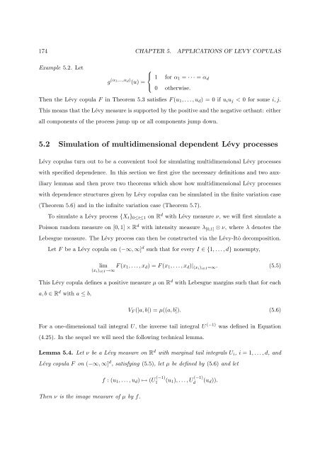
174 CHAPTER 5. APPLICATIONS OF LEVY COPULAS
Example 5.2. Let
⎧
⎨
g (α 1,...,α d ) 1 for α 1 = · · · = α d
(u) =
⎩
0 otherwise.
Then the Lévy copula F in Theorem 5.3 satisfies F (u 1 , . . . , u d ) = 0 if u i u j < 0 for some i, j.
This means that the Lévy measure is supported by the positive and the negative orthant: either
all components of the process jump up or all components jump down.
5.2 Simulation of multidimensional dependent Lévy processes
Lévy copulas turn out to be a convenient tool for simulating multidimensional Lévy processes
with specified dependence. In this section we first give the necessary definitions and two auxiliary
lemmas and then prove two theorems which show how multidimensional Lévy processes
with dependence structures given by Lévy copulas can be simulated in the finite variation case
(Theorem 5.6) and in the infinite variation case (Theorem 5.7).
To simulate a Lévy process {X t } 0≤t≤1 on R d with Lévy measure ν, we will first simulate a
Poisson random measure on [0, 1] × R d with intensity measure λ [0,1] ⊗ ν, where λ denotes the
Lebesgue measure. The Lévy process can then be constructed via the Lévy-Itô decomposition.
Let F be a Lévy copula on (−∞, ∞] d such that for every I ∈ {1, . . . , d} nonempty,
lim F (x 1, . . . , x d ) = F (x 1 , . . . , x d )| (xi ) i∈I =∞. (5.5)
(x i ) i∈I →∞
This Lévy copula defines a positive measure µ on R d with Lebesgue margins such that for each
a, b ∈ R d with a ≤ b,
V F (|a, b|) = µ((a, b]). (5.6)
For a one-dimensional tail integral U, the inverse tail integral U (−1) was defined in Equation
(4.25). In the sequel we will need the following technical lemma.
Lemma 5.4. Let ν be a Lévy measure on R d with marginal tail integrals U i , i = 1, . . . , d, and
Lévy copula F on (−∞, ∞] d , satisfying (5.5), let µ be defined by (5.6) and let
Then ν is the image measure of µ by f.
f : (u 1 , . . . , u d ) ↦→ (U (−1)
1 (u 1 ), . . . , U (−1)
d
(u d )).