Processus de Lévy en Finance - Laboratoire de Probabilités et ...

2.1. LEAST SQUARES CALIBRATION 61
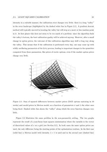
intensity in a suitable manner, the calibration error changes very little: there is a long “valley”
in the error landscape (highlighted by the dashed white line in Figure 2.1). A gradient descent
method will typically succeed in locating the valley but will stop at a more or less random point
in it. At first glance this does not seem to be too much of a problem: since the algorithm finds
the valley’s bottom, the best calibration quality will be achieved anyway. However, after a small
change in option prices, the outcome of this calibration algorithm may shift a long way along
the valley. This means that if the calibration is performed every day, one may come up with
wildly oscillating parameters of the Lévy process, leading to important changes in the quantities
computed from these parameters, like prices of exotic options, even if the market option prices
change very little.
3
x 10 5
2.5
2
1.5
1
0.5
0
2
1.5
1
λ
0.5
0
0.1
0.12
0.14
σ
0.16
0.18
0.2
Figure 2.1: Sum of squared differences between market prices (DAX options maturing in 10
weeks) and model prices in Merton model, as a function of parameters σ and λ the other ones
being fixed. Dashed white line shows the “valley” along which the error function changes very
little.
Figure 2.2 illustrates the same problem in the non-parametric setting. The two graphs
represent the result of a non-linear least squares minimization where the variable is the vector
of discretized values of ν on a grid (see Section 3.1). In both cases the same option prices are
used, the only difference being the starting points of the optimization routines. In the first case
(solid line) a Merton model with intensity λ = 1 is used and in the second case (dashed line)