Prospective crime mapping in operational context Final report

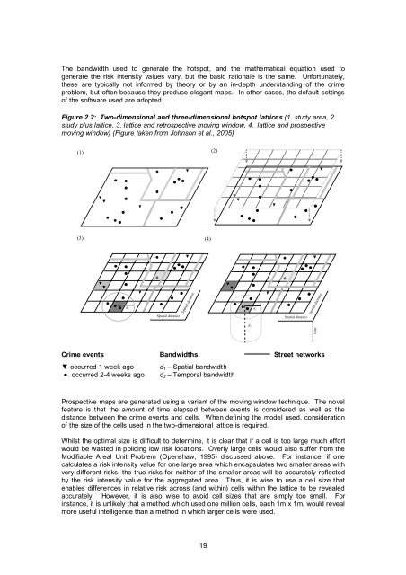
The bandwidth used to generate the hotspot, and the mathematical equation used togenerate the risk intensity values vary, but the basic rationale is the same. Unfortunately,these are typically not informed by theory or by an in-depth understanding of the crimeproblem, but often because they produce elegant maps. In other cases, the default settingsof the software used are adopted.Figure 2.2: Two-dimensional and three-dimensional hotspot lattices (1. study area, 2.study plus lattice, 3. lattice and retrospective moving window, 4. lattice and prospectivemoving window) (Figure taken from Johnson et al., 2005)(1) (2)(3)(4)d 1Spatial distanceSpatial distanced 2d 1Spatial distanceSpatial distancetimeCrime events Bandwidths Street networks▼ occurred 1 week ago d 1 – Spatial bandwidth● occurred 2-4 weeks ago d 2 – Temporal bandwidthProspective maps are generated using a variant of the moving window technique. The novelfeature is that the amount of time elapsed between events is considered as well as thedistance between the crime events and cells. When defining the model used, considerationof the size of the cells used in the two-dimensional lattice is required.Whilst the optimal size is difficult to determine, it is clear that if a cell is too large much effortwould be wasted in policing low risk locations. Overly large cells would also suffer from theModifiable Areal Unit Problem (Openshaw, 1995) discussed above. For instance, if onecalculates a risk intensity value for one large area which encapsulates two smaller areas withvery different risks, the true risks for neither of the smaller areas will be accurately reflectedby the risk intensity value for the aggregated area. Thus, it is wise to use a cell size thatenables differences in relative risk across (and within) cells within the lattice to be revealedaccurately. However, it is also wise to avoid cell sizes that are simply too small. Forinstance, it is unlikely that a method which used one million cells, each 1m x 1m, would revealmore useful intelligence than a method in which larger cells were used.19