Prospective crime mapping in operational context Final report

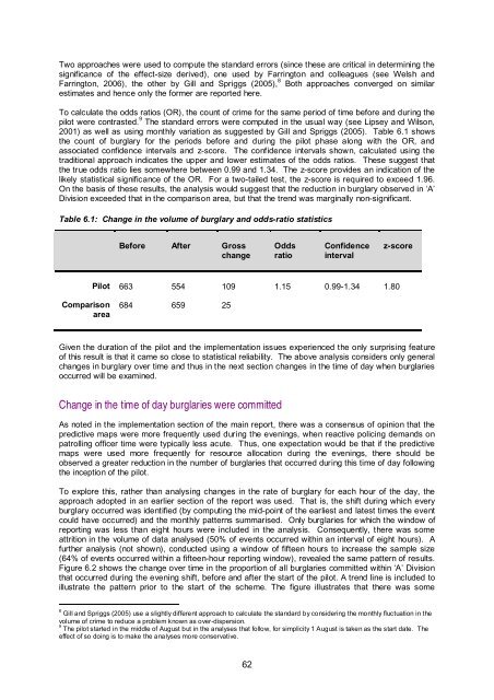
Two approaches were used to compute the standard errors (since these are critical in determining thesignificance of the effect-size derived), one used by Farrington and colleagues (see Welsh andFarrington, 2006), the other by Gill and Spriggs (2005), 8 Both approaches converged on similarestimates and hence only the former are reported here.To calculate the odds ratios (OR), the count of crime for the same period of time before and during thepilot were contrasted. 9 The standard errors were computed in the usual way (see Lipsey and Wilson,2001) as well as using monthly variation as suggested by Gill and Spriggs (2005). Table 6.1 showsthe count of burglary for the periods before and during the pilot phase along with the OR, andassociated confidence intervals and z-score. The confidence intervals shown, calculated using thetraditional approach indicates the upper and lower estimates of the odds ratios. These suggest thatthe true odds ratio lies somewhere between 0.99 and 1.34. The z-score provides an indication of thelikely statistical significance of the OR. For a two-tailed test, the z-score is required to exceed 1.96.On the basis of these results, the analysis would suggest that the reduction in burglary observed in ‘A’Division exceeded that in the comparison area, but that the trend was marginally non-significant.Table 6.1: Change in the volume of burglary and odds-ratio statisticsBefore After GrosschangeOddsratioConfidenceintervalz-scorePilot 663 554 109 1.15 0.99-1.34 1.80Comparisonarea684 659 25Given the duration of the pilot and the implementation issues experienced the only surprising featureof this result is that it came so close to statistical reliability. The above analysis considers only generalchanges in burglary over time and thus in the next section changes in the time of day when burglariesoccurred will be examined.Change in the time of day burglaries were committedAs noted in the implementation section of the main report, there was a consensus of opinion that thepredictive maps were more frequently used during the evenings, when reactive policing demands onpatrolling officer time were typically less acute. Thus, one expectation would be that if the predictivemaps were used more frequently for resource allocation during the evenings, there should beobserved a greater reduction in the number of burglaries that occurred during this time of day followingthe inception of the pilot.To explore this, rather than analysing changes in the rate of burglary for each hour of the day, theapproach adopted in an earlier section of the report was used. That is, the shift during which everyburglary occurred was identified (by computing the mid-point of the earliest and latest times the eventcould have occurred) and the monthly patterns summarised. Only burglaries for which the window ofreporting was less than eight hours were included in the analysis. Consequently, there was someattrition in the volume of data analysed (50% of events occurred within an interval of eight hours). Afurther analysis (not shown), conducted using a window of fifteen hours to increase the sample size(64% of events occurred within a fifteen-hour reporting window), revealed the same pattern of results.Figure 6.2 shows the change over time in the proportion of all burglaries committed within ‘A’ Divisionthat occurred during the evening shift, before and after the start of the pilot. A trend line is included toillustrate the pattern prior to the start of the scheme. The figure illustrates that there was some8 Gill and Spriggs (2005) use a slightly different approach to calculate the standard by considering the monthly fluctuation in thevolume of crime to reduce a problem known as over-dispersion.9 The pilot started in the middle of August but in the analyses that follow, for simplicity 1 August is taken as the start date. Theeffect of so doing is to make the analyses more conservative.62