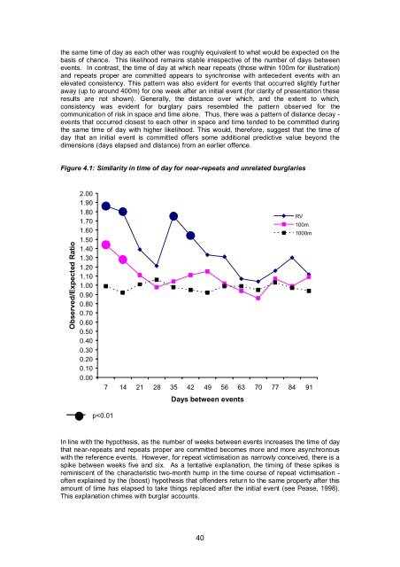
Time of day consistency?As noted above, a further question raised was whether burglaries that occur very close toeach other <strong>in</strong> space and time (with<strong>in</strong> a few days) are committed at the same time of dayusually with<strong>in</strong> the same police shift as each other? The fact that hotspots change accord<strong>in</strong>g toshift (e.g. see Ratcliffe 2002) <strong>in</strong>cl<strong>in</strong>es one to that view, but a more direct test was sought. Anaffirmative set of results would suggest that a burglary not only confers risk for a particulargeography and duration, but also for a specific time of day (morn<strong>in</strong>g, afternoon or even<strong>in</strong>g).To illustrate, consider that an offender might have a preference for certa<strong>in</strong> activities dur<strong>in</strong>g theday (see Rengert and Wasilchick, 2000). Consequently, he/she may visit certa<strong>in</strong> locationsdur<strong>in</strong>g daytime hours. Whilst there, he/she may commit offences if the opportunity presentsitself. This rhythm of activity, if regular enough, means that an offender will be at certa<strong>in</strong>places at certa<strong>in</strong> times. If he/she chooses to commit <strong>crime</strong>s, and <strong>in</strong> particular near-repeats atthese locations, then one would expect to see some consistency <strong>in</strong> the time of day at whichburglaries are committed <strong>in</strong> those areas. Burglars would appear to work shifts.To exam<strong>in</strong>e this hypothesis, one year’s data (January-December 2004) were analysed for thepolice force area (N=8,968). Each <strong>crime</strong> was compared to every other and the number of<strong>crime</strong>s that occurred at different spatial and temporal <strong>in</strong>tervals identified. In l<strong>in</strong>e with theauthors’ earlier work, the spatial <strong>in</strong>tervals here used were multiples of 100m, and the temporal<strong>in</strong>tervals one week periods. Next, all events were compared to see if they occurred dur<strong>in</strong>g thesame police shift (7am to 3pm, 3pm to 10pm, or 10pm to 7am) and a cont<strong>in</strong>gency tablepopulated. Comparisons between events that occurred on the same day as each other wereexcluded from the analyses presented as their <strong>in</strong>clusion has the potential to <strong>in</strong>flate theconsistency observed 3 - as a <strong>crime</strong> series committed dur<strong>in</strong>g one even<strong>in</strong>g would naturally beconsistent <strong>in</strong> terms of the police shift dur<strong>in</strong>g which the events occurred as well as where theyoccurred.To determ<strong>in</strong>e dur<strong>in</strong>g which shift an event occurred, data concerned with the day and time ofeach burglary were analysed. Typically, most burglaries occur when a victim is away from theproperty. Accord<strong>in</strong>gly, rather than record<strong>in</strong>g a s<strong>in</strong>gle time at which a <strong>crime</strong> may have takenplace, the police ask for a likely time w<strong>in</strong>dow, expressed as the earliest time to the latest timethe burglary could have occurred. This was mentioned earlier as a qualification on theanalysis of <strong>crime</strong>s by shift. In the analysis that follows, the midpo<strong>in</strong>t of these two times wasused as an <strong>in</strong>dicator of the time of the event. Crimes were excluded from the analysis if thetime w<strong>in</strong>dow (for the earliest and latest day and times) exceeded 15 hours. Follow-upanalyses used shorter <strong>in</strong>tervals of four and eight hours, and revealed the same pattern ofresults.To determ<strong>in</strong>e whether the emergent patterns differed from what would be expected on thebasis of chance, if the time of day that near-repeat burglaries were committed were unrelated,Monte-Carlo simulation was used to generate a chance distribution. To do this, us<strong>in</strong>g apseudo-random number generator, each <strong>crime</strong> was randomly assigned the police shift for adifferent burglary (each shift was reassigned only once), and a new cont<strong>in</strong>gency tablederived. This was completed 999 times. If the observed results represent a statisticallysignificant pattern, then one would expect that for any space-time comb<strong>in</strong>ation (e.g. eventsthat occurred with<strong>in</strong> 100m and seven days of each other) the number of burglaries for whichthe shifts are concordant would be greater than the Monte-Carlo results for at least 95 percent of the simulations. This equates to a threshold of statistical significance at the five percent level. In this analysis, as so many comparisons were made, the more conservative oneper cent level of statistical significance was adopted.A subset of the results, shown as Figure 4.1, are presented as the ratio of the observednumber of burglary pairs for which the events occurred dur<strong>in</strong>g the same time of day (shift),divided by the mean of the Monte-Carlo simulations. Thus, a value of one would <strong>in</strong>dicate thatthe observed value was equal to that expected. Statistically significant results are highlightedwith exaggerated markers on the graph. The dotted l<strong>in</strong>e shows that for events which occurredbetween 1,000m of each other, the observed number of burglary pairs that occurred dur<strong>in</strong>g3 Analyses which <strong>in</strong>cluded such comparisons produced an identical pattern of results.39
the same time of day as each other was roughly equivalent to what would be expected on thebasis of chance. This likelihood rema<strong>in</strong>s stable irrespective of the number of days betweenevents. In contrast, the time of day at which near repeats (those with<strong>in</strong> 100m for illustration)and repeats proper are committed appears to synchronise with antecedent events with anelevated consistency. This pattern was also evident for events that occurred slightly furtheraway (up to around 400m) for one week after an <strong>in</strong>itial event (for clarity of presentation theseresults are not shown). Generally, the distance over which, and the extent to which,consistency was evident for burglary pairs resembled the pattern observed for thecommunication of risk <strong>in</strong> space and time alone. Thus, there was a pattern of distance decay -events that occurred closest to each other <strong>in</strong> space and time tended to be committed dur<strong>in</strong>gthe same time of day with higher likelihood. This would, therefore, suggest that the time ofday that an <strong>in</strong>itial event is committed offers some additional predictive value beyond thedimensions (days elapsed and distance) from an earlier offence.Figure 4.1: Similarity <strong>in</strong> time of day for near-repeats and unrelated burglariesObserved/Expected Ratio2.001.901.801.701.601.501.401.301.201.101.000.900.800.700.600.500.400.300.200.100.00RV100m1000m7 14 21 28 35 42 49 56 63 70 77 84 91Days between eventsp
- Page 2 and 3: 1. UCL JILL DANDO INSTITUTE OF CRIM
- Page 4 and 5: ContentsAcknowledgementsExecutive s
- Page 6 and 7: 2.5 Illustration of a simple neares
- Page 8 and 9: Project outcomesPatterns of burglar
- Page 10 and 11: those that involved collaboration w
- Page 12 and 13: 1. IntroductionThis report represen
- Page 14 and 15: optimally calibrated system, the go
- Page 16 and 17: e ij = n .j x n i.nWhere, e ij is t
- Page 18 and 19: Table 2.2: Knox ratios for Mansfiel
- Page 20 and 21: Table 2.6: Monte-Carlo results for
- Page 22 and 23: Table 2.10: Weekly Knox ratios for
- Page 24 and 25: Table 2.14: Monte-Carlo results for
- Page 26 and 27: Figure 2.1: The five policing areas
- Page 28 and 29: The results for area 5 again demons
- Page 30 and 31: The bandwidth used to generate the
- Page 32: a densely populated urban area this
- Page 35 and 36: Table 2.24: Average number of crime
- Page 37 and 38: Patrolling efficiencyAs discussed e
- Page 39 and 40: 3. Tactical options and selecting a
- Page 41 and 42: Selecting a pilot siteThe decision
- Page 43 and 44: Table 3.2: Tactical options matrixT
- Page 45 and 46: Type ofinterventionStudyUse ofintel
- Page 47 and 48: Other potential tactical optionsAt
- Page 49: 4. System development and evolution
- Page 53 and 54: unfortunately, implementation or us
- Page 55 and 56: any tactical options were employed
- Page 57 and 58: the end of the pilot. In addition t
- Page 59 and 60: Figure 5.1: Promap dissemination pr
- Page 61 and 62: the busy schedule of the new Divisi
- Page 63 and 64: Tactical deliveryCommand Team daily
- Page 65 and 66: Table 5.3: Number of respondents wh
- Page 67 and 68: permitted, up to four plain clothed
- Page 69 and 70: observation made by those who used
- Page 71 and 72: A simple time-series analysis (see
- Page 73 and 74: Two approaches were used to compute
- Page 75 and 76: Figure 6.3: Changes in the proporti
- Page 77 and 78: Figure 6.5: Changes in the proporti
- Page 79 and 80: With respect to implementation real
- Page 81 and 82: ReferencesAggresti, A. (1996) An In
- Page 83 and 84: Johnson, S.D., Summers, L., and Pea
- Page 85 and 86: Appendix 1. The information technol
- Page 87 and 88: Figure A1.2: Stand-alone applicatio
- Page 89 and 90: Recommendations that may be realise
- Page 91 and 92: Section 1: knowledge and understand
- Page 93 and 94: Extra Comments (please outline any
- Page 95 and 96: In relation to the evaluation of in
- Page 97 and 98: Time-series analysisFor the purpose
- Page 99 and 100: Figure A3.1: Changes in the spatial
- Page 101 and 102:
Figure A3.2: Lorenz curves showing
- Page 103 and 104:
To recapitulate and elaborate, the
- Page 105 and 106:
Concluding comments on methodThe te
- Page 107 and 108:
Figure A5.2: An enlargement of the
- Page 109 and 110:
Figure A5.6: Prospective map magnif
- Page 111:
Produced by the Research Developmen