Prospective crime mapping in operational context Final report

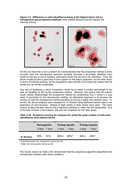
Figure 2.4: Differences in cells identified as being at the highest future risk byretrospective and prospective methods (cells shaded darkest have the highest riskintensity values)On the one hand this is not a problem as it demonstrates that the prospective method is moreaccurate than the retrospective approach probably because it accurately identifies morelocations that are at risk of burglary, particularly those that are yet to be victimised. Thus, theabove results provide a good test of and support for the theory proposed. On the other hand,in terms of practical policing, as the prospective maps identify more areas this means that theresults are not strictly comparable.One way of facilitating a direct comparison would be to select a smaller percentage of thecells as identified at risk by the prospective method. However, this means that the authorswould unfairly disadvantage the prospective method by constraining how it works in a waywhich is precluded for the retrospective method. An alternative approach is to increase thenumber of cells the retrospective method identifies as having a higher risk intensity value. Todo this, the above analyses were repeated for ‘A’ Division using additional historic data in thegeneration of each forecast. Instead of eight weeks of data, twelve were used. The samevolume of data was also used for the prospective methods to make the test comparable. Dueto the time involved in the analysis, this was not completed for the other areas.Table 2.26: Predictive accuracy for analyses for which the same number of cells wereidentified by each method (N=22)Retrospective Promap specific Promap (classic)2 days 7 days 2 days 7 days 2 days 7 days‘A’ Division 58% 61% 66%+ 66%* 64%+ 64%** Significantly better than retrospective method (p