Guide to COST-BENEFIT ANALYSIS of investment projects - Ramiri

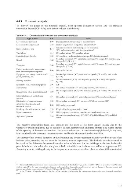
4.4.3 Economic analysisTo convert the prices in the financial analysis, both specific conversion factors and the standardconversion factor (SCF=0.96) have been used (see table below).Table 4.41 Conversion factors for the economic analysisType of cost CF NotesLabour: skilled personnel 1.00 The labour market is assumed to be competitiveLabour: unskilled personnel 0.60 Shadow wage for not-competitive labour market 93Expropriation or land 1.34Standard conversion factor multiplied for local price(40% higher than prices paid for expropriation)Yard labour 0.64 10% skilled labour, 90% unskilled labourMaterials for civil works 0.83 55% machinery and manufactured goods, 45% building materialsRentals 0.683% skilled personnel, 37% unskilled personnel, 30% energy, 20% maintenance,10% profits 94 (CF = 0)Transport 0.683% skilled personnel, 37% unskilled personnel, 30% energy, 20% maintenance,10% profits (CF = 0)Project studies, works management,trials and other general expenses1.00 100% skilled labourEquipment, machinery, manufactured 50% local production (SCF), 40% imported goods (CF = 0.85), 10% profits0.82goods, carpentry, etc.(CF = 0)Building materials 0.8575% local materials (SCF), 15% imported goods (CF = 0.85), 10% profits(CF = 0)Electricity, fuels, other energy prices 0.96 SCFMaintenance 0.71 15% skilled personnel, 65% unskilled personnel, 20% materialsReagents and other specialist materials 0.8030% local production (SCF), 60% imported goods (CF = 0.85), 10% profits (CF= 0)Intermediate goods and technicalservices0.71 10% skilled personnel, 60% unskilled personnel, 30% manufactured goodsElimination of treatment sludge 0.80 30% unskilled personnel, 20% transport, 50% local services (SCF)Administrative, financial andeconomic services1.00 100% skilled personnelResulting value of investment costs 0.76 Weighted by the types of project costsReplacement costs 0.82 100% equipment, machinery, manufactured goods, carpentry, etc.Agricultural product 0.8568% various agricultural input (CF=SCF), 2% skilled labour, 30% unskilledlabourThe negative externalities taken into account are: the costs of the local impact (mainly due to thewastewater treatment plants) due to the noise, odours, aesthetic and landscape impact. The overall impactof the opening of the construction sites - in an extra urban area - is considered negligible and, in any case,it is absorbed by the corrected investment costs and by the aforementioned externalities.The impact of the normal operation of the depurator and tertiary treatment plant is valued by means of anhedonic price, assuming the real estate in the nearby area are depreciated. The hedonic price is assumed tobe equal to the difference between the market value of the rent for the buildings in the area before theplant is built and the value after the plant is built; this difference is then corrected by an appropriate CF.Assuming a mean building density in the impact area (an area, centred on plant, of about 600 m radius) of93The unskilled labour conversion factor is calculated on the basis of the shadow wage, as follows: SW = FW x (1-u) x (1-t), were SW is theshadow wage, SW in the wage assumed in the financial analysis, u is local (regional) unemployment rate and t is the rate of the social security andrelevant taxes. In the case study, set u=12% and t=32%, the CF (SW/FW) is equal to 0.60.94In the CF table, ‘10% profits’ indicates the share of the company profits among the various costs, that contribute to the overall cost of thegood.173