Guide to COST-BENEFIT ANALYSIS of investment projects - Ramiri

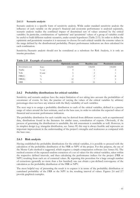
2.6.1.1 Scenario analysisScenario analysis is a specific form of sensitivity analysis. While under standard sensitivity analysis theinfluence of each variable on the project’s financial and economic performance is analysed separately,scenario analysis studies the combined impact of determined sets of values assumed by the criticalvariables. In particular, combinations of ‘optimistic’ and ‘pessimistic’ values of a group of variables couldbe useful to build different realistic scenarios, under certain hypotheses (Table 2.15). In order to define theoptimistic and pessimistic scenarios it is necessary to choose for each critical variable the extreme values inthe range defined by the distributional probability. Project performance indicators are then calculated foreach combination.Sensitivity/Scenario analysis should not be considered as a substitute for Risk Analysis, it is only aninterim procedure.Table 2.15 Example of scenario analysisOptimistic scenario Baseline case Pessimistic scenarioInvestment cost Euro 125,000 130,000 150,000Traffic % var 9 5 2Tolls €/unit 5 2 1FRR(C) % 2 -2 -8FRR(K) % 12 7 2ERR % 23 15 62.6.2 Probability distributions for critical variablesSensitivity and scenario analyses have the major limitation of not taking into account the probabilities ofoccurrence of events. In fact, the practice of varying the values of the critical variables by arbitrarypercentages does not have any relation with the likely variability of such variables.The next step is to assign a probability distribution to each of the critical variables, defined in a preciserange of values around the best estimate, used as the base case, in order to calculate the expected values offinancial and economic performance indicators.The probability distribution for each variable may be derived from different sources, such as experimentaldata, distributions found in the literature for similar cases, consultation of experts. Obviously, if theprocess of generating the distributions is unreliable, the risk assessment is unreliable as well. However, inits simplest design (e.g. triangular distribution, see Annex H) this step is always feasible and represents animportant improvement in the understanding of the project’s strengths and weaknesses as compared withthe base case.2.6.3 Risk analysisHaving established the probability distributions for the critical variables, it is possible to proceed with thecalculation of the probability distribution of the FRR or NPV of the project. For this purpose, the use ofthe Monte Carlo method is suggested, which requires a simple computation software (see Annex H). Themethod consists of the repeated random extraction of a set of values for the critical variables, taken withinthe respective defined intervals, and then calculating the performance indices for the project (FRR orNPV) resulting from each set of extracted values. By repeating this procedure for a large enough numberof extractions (generally no more than a few hundred) one can obtain a pre-defined convergence of thecalculation as the probability distribution of the FRR or NPV.The most helpful way of presenting the result is to express it in terms of the probability distribution orcumulated probability of the FRR or the NPV in the resulting interval of values. Figures 2.6 and 2.7provide graphical examples.61