Guide to COST-BENEFIT ANALYSIS of investment projects - Ramiri

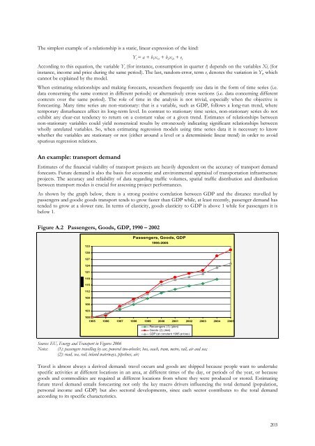
The simplest example of a relationship is a static, linear expression of the kind:Y t = a + b 1 x 1t + b 2 x 2t + e tAccording to this equation, the variable Y t (for instance, consumption in quarter t) depends on the variables Xi t (forinstance, income and price during the same period). The last, random-error, term e t denotes the variation in Y t , whichcannot be explained by the model.When estimating relationships and making forecasts, researchers frequently use data in the form of time series (i.e.data concerning the same context in different periods) or alternatively cross sections (i.e. data concerning differentcontexts over the same period). The role of time in the analysis is not trivial, especially when the objective isforecasting. Many time series are non-stationary: that is a variable, such as GDP, follows a long-run trend, wheretemporary disturbances affect its long-term level. In contrast to stationary time series, non-stationary series do notexhibit any clear-cut tendency to return on a constant value or a given trend. Estimates of relationships betweennon-stationary variables could yield nonsensical results by erroneously indicating significant relationships betweenwholly unrelated variables. So, when estimating regression models using time series data it is necessary to knowwhether the variables are stationary or not (either around a level or a deterministic linear trend) in order to avoidspurious regression relations.An example: transport demandEstimates of the financial viability of transport projects are heavily dependent on the accuracy of transport demandforecasts. Future demand is also the basis for economic and environmental appraisal of transportation infrastructureprojects. The accuracy and reliability of data regarding traffic volumes, spatial traffic distribution and distributionbetween transport modes is crucial for assessing project performances.As shown by the graph below, there is a strong positive correlation between GDP and the distance travelled bypassengers and goods: goods transport tends to grow faster than GDP while, at least recently, passenger demand hastended to grow at a slower rate. In terms of elasticity, goods elasticity to GDP is above 1 while for passengers it isbelow 1.Figure A.2 Passengers, Goods, GDP, 1990 – 2002133Passengers, Goods, GDP1995-20051301271241211181151121091061031001995 1996 1997 1998 1999 2000 2001 2002 2003 2004 2005Passengers (1) (pkm)Goods (2) (tkm)GDP (at constant 1995 prices)Source: EU, Energy and Transport in Figures 2006Notes: (1): passengers travelling by car, powered two-wheeler, bus, coach, tram, metro, rail, air and sea;(2): road, sea, rail, inland waterways, pipelines, air;Travel is almost always a derived demand: travel occurs and goods are shipped because people want to undertakespecific activities at different locations in an area, at different times of the day, or periods of the year, or becausegoods and commodities are required at different locations from where they were produced or stored. Estimatingfuture travel demand entails forecasting not only the key macro drivers influencing the total demand (population,personal income and GDP) but also sectoral developments, since each sector contributes to the total demandaccording to its specific characteristics.203